Estimating at unsampled locations

TL;DR

The basic problem is to estimate value at an unsampled location by combining nearby observations. In geostatistics, this process is formalized as Kriging (spatial regression, locally weighted regression, Gaussian processes, etc.). There are many types of ‘Kriging’ algorithms. Simple and ordinary kriging are popular versions. But the underlying process is identical; define some notion of ‘optimal’ and solve for weights to combine the nearby data into the ‘optimal’ estimate at the unsampled location.

Introduction

The motivation for geostatistics is to estimate the value of some interesting variable at an unsampled location. This is extremely important in mining and mineral resources since sampling is crazy expensive and geological variables are often continuous along known orientations.

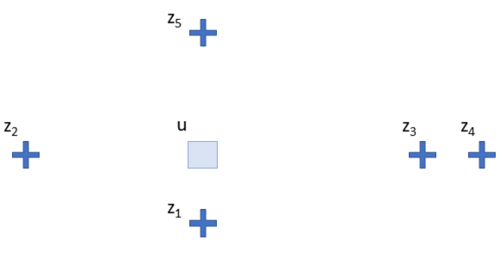
Fig 1: A scenario with spatially located samples and a single unsampled location.

The most popular strategy for estimating at unsampled locations is to combine the value of samples at nearby locations by giving some weight to each sample and taking the sum over all samples. Consider the simple case below; we have 4 locations (the $z$) and one unsampled location $\Box$ where we are going to make an estimate:

This estimate becomes a weighted combination of the values at each location, e.g.:

$$ \Box = \lambda_1 * z_1 + \lambda_2 * z_2 + \lambda_3 * z_3 + \lambda_4 * z_4 $$

Which is generalized to any number of nearby locations $N$ as:

$$ z^*(\mathbf{u}{\Box}) = \sum{i=1}^N \lambda_i z(\mathbf{u}_i) $$

Where $\lambda_i$ are weights, $z(\mathbf{u}_i)$ are the sample values at different $\mathbf{u}_i$ locations.

Basic Spatial Estimators

Nearest Neighbor

The most basic (and somehow still used) version of this is to search for only the closest neighbor and give all the weight to that observation. This is called nearest neighbor (NN) estimation. In the above case this means that $z_1$ is the only location to influence the estimate. As you can imagine, there are issues with this… but it might be reasonable with dense sampling, and is useful as a check on more complex strategies that might unfairly extrapolate.

Inverse Distance Weighted

Another common strategy is to calculate inverse-distance weights (IDW), where the weight given to each sample is inversely proportional to the distance between the samples and unsampled location:

$$ \lambda_i = \frac{1}{d_{i\Box}} $$

In this case $d_{i\Box}$ is the distance between the $i^{th}$ location and the location being estimated $\Box$. This strategy is better than taking the nearest data since we are allowing more nearby data to influence the estimate, but still falls short of other methods that can account for observed spatial continuity of the underlying variable.

Kriging

Kriging methods differ from other interpolation methods with 3 main properties:

1. The Variogram

Kriging uses a model of spatial continuity calculated from the sample data (the variogram). The variogram captures the relationship between locations separated by a certain distance and direction. Details are beyond the scope (and covered elsewhere), but the result of variogram calculation and modeling is a model that describes continuity as a function of distance and direction.

2. Optimality

The base theoretically valid kriging is called simple kriging (SK), where ‘optimal’ is an estimate with the minimum mean-squared error (MSE):

$$ \lambda \quad S.T. \quad min [ E{ [ z^*_{\Box} - z ]^2 } ] $$

If a estimate is required at a location beyond the range of influence of nearby data (as per the variogram model) then, without other information, the best estimate is the mean of the dataset.

3. Relationships Between Nearby Locations

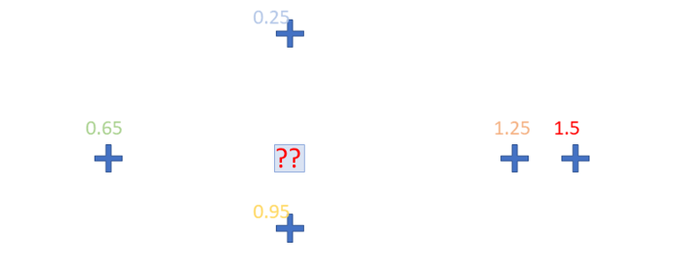
Kriging allows the nearby data to influence how other nearby data inform the unsampled location (e.g., screening). Considier the following zoomed view from Fig. 1:

Fig 2: Zoomed view of Fig. 1 showing clustered sampling and a case of screening.

The weights calculated by kriging will account for the fact that $z_3$ and $z_4$ are highly related to one another and along the same orientation. That is, location $z_3$ will be given a large weight and effectively ‘screens’ location $z_4$ for estimating at the unsampled location. This amounts to a sort of declustering; the tightly spaced $z_3$ and $z_4$ are effectively considered a single location, so the estimate would be (roughly) 50% from location $z_2$ and 50% from the combined $z_3$ and $z_4$. Contrast this with IDW in this scenario; since the distances are all similar, roughly 33% of the weight would be given to each location, which may unfairly bias the estimate.

Ordinary Kriging

Ordinary Kriging (OK) is the bread and butter of the mining industry. OK uses the same optimality criteria as SK, but additionally constrains the sum of the weights to be 1 such that no weight is given to the local mean:

$$ \mathbf{\lambda} \quad S.T. \quad min [ E{ [ z^*_{\Box} - z ]^2 } ] $$

$$ \sum_{i=1}^N \lambda_i = 1 $$

Under this constraint, the mean is locally re-estimated. Though this is an extremely useful property of OK, the additional constraint placed on the estimate means that other optimal properties of the estimate (minimum error variance) are no longer met (Fig. 3).

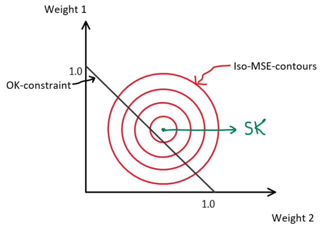
Fig 3: For a case of estimating from 2 sample data, the minimum MSE is given by the SK estimate; any constraints placed on the estimator result in an increased error (MinE612, University of Alberta).

Other Kriging Types

Well, there are many other types of kriging. Rossi and Deutsch (2014) list 13 types, and most of those can also be used in co-mode (> 1 spatially correlated variables). Five of these types are variations on OK where the unknown local mean is obtained through other interesting methods; the most well known is Universal Kriging (see Rossi and Deutsch for details). The rest modify how value is represented at the unsampled locations (e.g., a distribution instead of a single value).

Should you care? I’d say no. Sure, each type of Kriging will find application in some of the many geological domains out there, but the CORRECT estimate at the unsampled location is generated with SK in a stationary domain under a Gaussian assumption; a scenario called multiGaussian kriging (MGK). If you’ve met the conditions to make MGK applicable to your problem, then you’d better be considering simulation since you’ve already done the hard work. But… in practice meeting these conditions is difficult and involves lots of assumptions, and blindly assuming these are met and continuing on with the workflow leads to many problems… So MGK, simulation and other probabilistic methods aren’t seeing widespread adoption in mining (see: Silva and Bosivert, 2014).

What’s the Takeaway??

In mining, OK is the main estimator, with the search strategy used as a dial to tweak estimates to different applications (short term, interim, long term, etc). However, acquiring some measure of uncertainty is increasingly desired. As seen above, OK does not give the minimum error variance. Instead, SK needs to be applied for applications where this property is required. Things like recoverable reserves at different production volumes, the probability to be above a cutoff, etc., must be characterized with methods that treat value at the unsampled location as a distribution and not a single value.

References/Resources

• Rossi, M. E., and C. V. Deutsch. Mineral Resource Estimation. Springer Science, 2014. https://doi.org/10.1007/978-1-4020-5717-5.

• Silva, D., and J. B. Boisvert. “Mineral Resource Classification: A Comparison of New and Existing Techniques.” Journal of the South African Institute of Mining and Metallurgy 114, no. 3 (2014): 265–73.