The Proportional Effect and Its Affect

So you understand what the proportional effect is, and thus what heteroscedasticity is (If not, head on over to our previous post here)! Now let’s dive into how this can affect our modeling of the data.

TL;DR

If we have heteroscedastic data, then our data won’t behave consistently. The closer ranges of the variogram will be affected the most by the proportional effect.

Therefore Know thy data! Many modeling algorithms assume “well behaved data” (read: homoscedastic, known and constant mean, other fun non-existent-in-reality properties…). Skewed distributions are very common for geological variables, thus, you will probably have to account for the proportional effect somehow somewhere in your workflow. If you don’t account for it, then errors will build upon errors as you travel down the rabbit hole!

The Proportional Effect And Its Affect On The Variogram

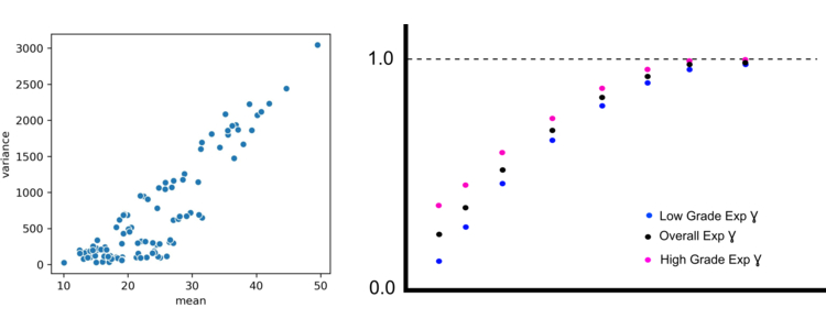
Whether modeling in original units or doing some volume variance calculations, there will be periods in our lives where we need a variogram. When calculating the experimental variogram with a large proportional effect present (highly heteroscedastic data), there are some things to note. The experimental variogram calculates the variability of your data at various distances (add link to variogram posts?). Most calculations for the experimental variogram (pair-wise relative being an exception) assumes the variability of the data is defined solely by the linear distance between two data locations, i.e. the lag distance. Ahah! That means we are assuming the data is homoscedastic, which is a slightly easier to say word meaning the opposite of heteroscedastic, AKA no proportional effect. However, if we know that our data shows the proportional effect, that means that the variogram model will depend not only on lag distance but also the location since the variance of your data will change depending on whether you are in a high value or low value zone. To highlight this, let’s look at a simple example.

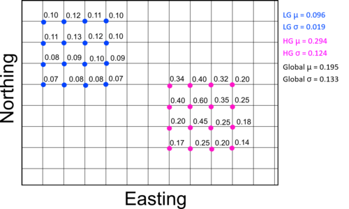
Fig 1: Simple example showing a significant proportional effect

Figure 1 shows a dataset that exhibits the proportional effect. If we focus on a high grade zone (Magenta) and a low grade zone (Blue) we can calculate the experimental variogram for a short lag distance (say h = 2 cells) for each zone separately. The blue variogram in this case would give us a gamma_h2 value of 0.0003, while the Magenta variogram would give us a higher gamma_h2 of 0.0154. If we calculate the variogram across the whole domain we would end up with an overall gamma_h2 of 0.0078. This means that we will end up over estimating how variable the mineral grades are in our low grade zones while underestimating how variable the grades are in the high grade zones. The variability will in fact be more pronounced in the shorter lag distances than it will be in the longer last distances. You would likely see something like Figure 2 of you plotted all three variograms

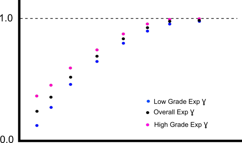
Fig 2: Local experimental variograms versus Domain experimental variogram

Therefore, if you are seeing the proportional effect in your data, then you might need to account for that. You might consider looking further into relational variograms that account for the proportional effect (which is complicated), or maybe think about transforming your data to a Gaussian distribution. Of course, maybe even doing something as simple as thinking a little more about your modelling domains could be enough.

SIDE NOTE: Why is it important if you are modeling in original units or not? Well, it turns out that a Gaussian transformation will almost always transform the data to be homoscedastic thus removing the proportional effect. The back transformation to original units will reintroduce heteroscedasticity. However, if you are still doing volume variance calculations, then those need to be done in original units and you will still need to be aware of the proportional effect.

Conventional volume variance calculations require a variogram model in original units to determine the variance at different volume supports. The calculation is done by subtracting the average variogram model at the larger volume of support (the scale you are interested in averaging up to) by the variogram at the smaller volume of support (the scale you are modeling at). However, we just pointed out that the normal variogram model is a function of only the lag distance, therefore this means that due to the proportional effect the local mean will also affect the variogram. What does this mean if you don’t consider the proportional effects affect on the variogram? It means that, in most cases, the dispersion variance will be too high and your volume variance calculation will be wrong.

Take Away

If you require a variogram model in original units and your data is heteroscedastic, consider using an algorithm such as the correlogram to calculate the experimental variogram, it handles heteroscedastic data well as it considers both lag distance and the local means at the head and tail. Otherwise, you can transform the data into the Gaussian distribution, model the variogram, and back-transform the variogram to original units.

Resources

• Manchuk, J., Leuangthong, O., Deutsch, C.V. (2009) Teacher’s aide: the proportional effect of spatial variables. Mathematical Geology, 41(7): 799-816
• Manchuk, J., Leuangthong, O., & Deutsch, C. V., (2006). A New Look at the Proportional Effect: what is it and how do we model it. Centre for Computational Geostatistics Report 8, 109. University of Alberta, Canada.
• Chiles J.P. and Delfiner P. (1999) Geostatistics Modeling Spatial Uncertainty, John Wiley and Sons, Inc.

Interested in learning more about variograms? Check out our “WTF is a variogram” series