Simple Kriging ≠ MGK
Simple Kriging ≠ MGK
TL;DR
Kriging gives us the best estimate by combining values at nearby locations. MultiGaussian kriging can be thought of as a recipe to cook up distributions of uncertainty given nearby data. This recipe includes: Gaussian transformation, simple kriging, and quantile back-transformation.
Introduction
We’ve (hopefully) all heard of probabilistic estimators in geostatistics, where the goal is to predict a probability distribution at the unsampled location (a node in an estimation grid). This distribution may be given by a number of observations (e.g., by Monte Carlo simulation), or it can be represented by a set of parameters such as a shape (e.g., lognormal), the expected value (mean), and some measure of the spread (variance).
MultiGaussian Kriging
The classical simple kriging (SK) formulation calculates weights that minimize the mean-squared error (MSE) between the estimate and the unknown truth at the unsampled location (kriging) . If we additionally assume the sample data follow a Gaussian distribution (which can be enforced with a quantile-to-quantile transformation), weights calculated by the simple kriging estimator can be used to define the mean and variance of a Gaussian distribution at the unsampled location. By estimating the parameters of the distribution, we now have a probabilistic estimate since it is a full distribution defining the probability of all possible estimates at that location. Under these Gaussian conditions, the estimator is referred to as multiGaussian kriging (MGK; or the normal equations).
However, there are special requirements for post-processing the estimated distribution. The key is to remember that the estimate defines a full distribution, not a single value, and that distribution must be treated accordingly.
Gaussian Transform
The normal scores (NS) transform is an absolute requirement of MGK. That is, through quantile-to-quantile (QQ) transform we take an arbitrarily distributed (usually lognormal) variable and enforce the distribution to be univariate Gaussian (seriously check this out if there are lingering questions!):
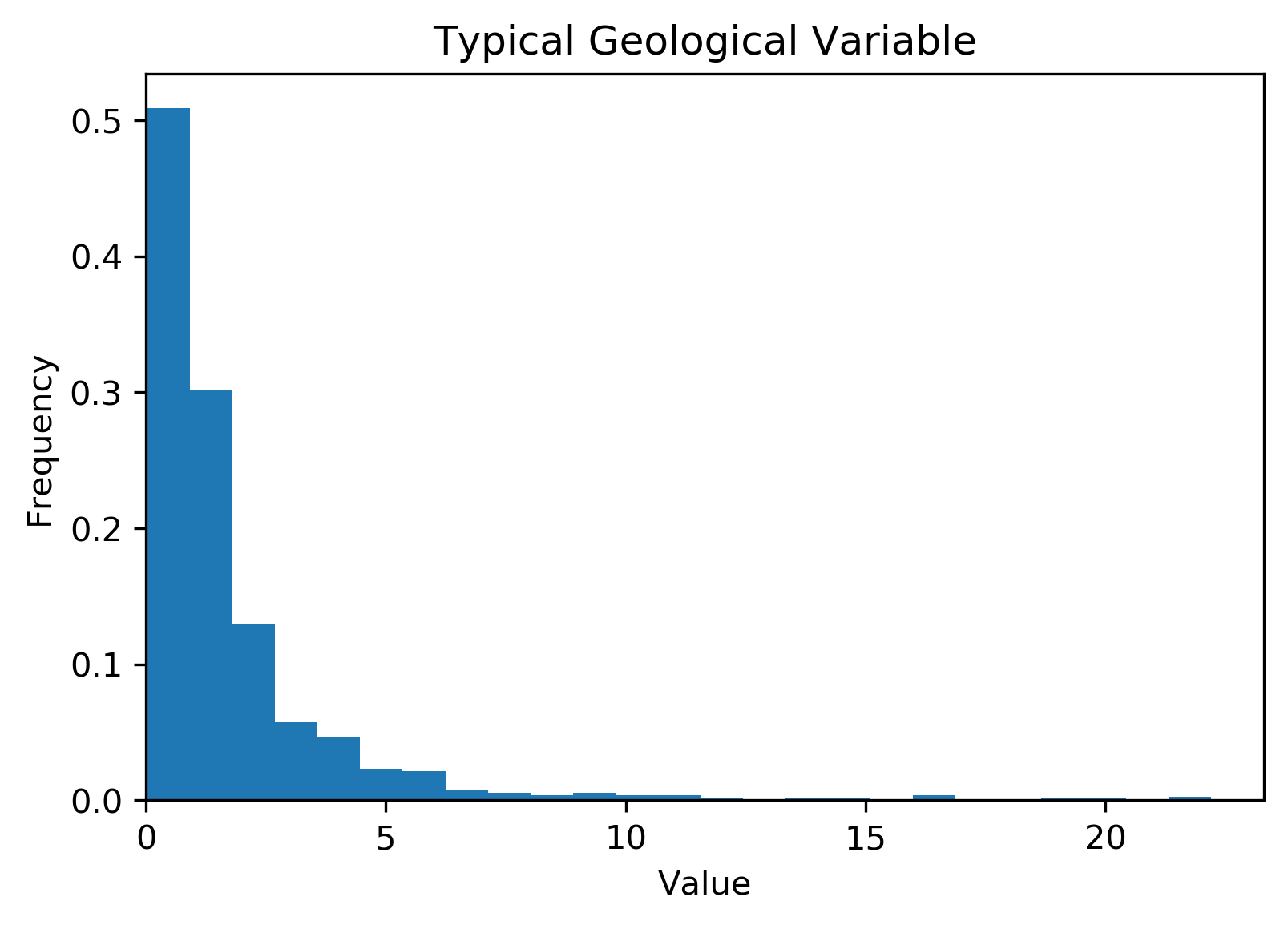
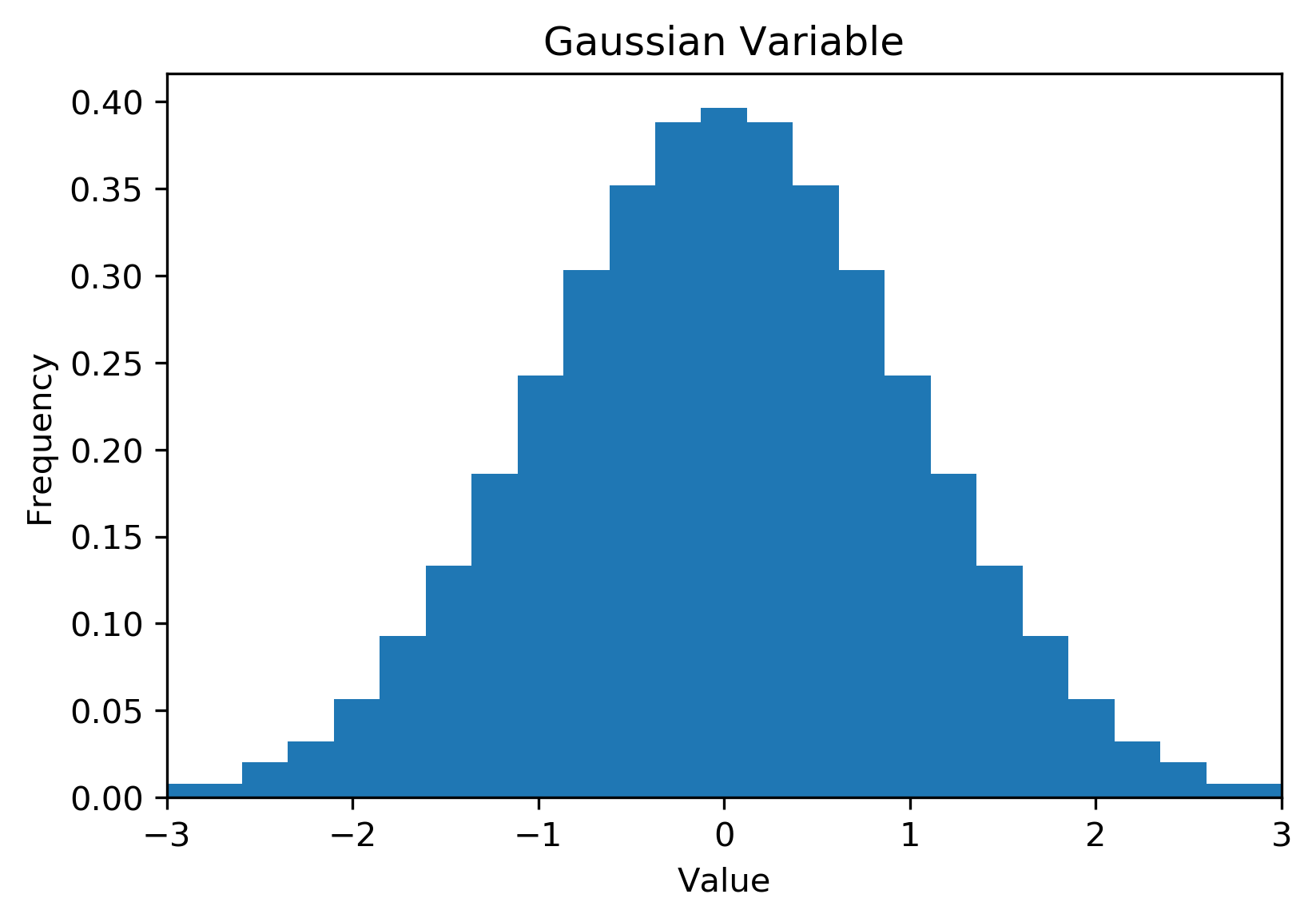
Fig. 1: A lognormal variable (left) and the Gaussian transformed variable (right).
But the ‘multi’ part of MGK is actually referring to the set of all possible distributions at all possible locations in the domain, and how all of those are Gaussian. Thinking about the sample locations where we have a measured value, there is no distribution at those locations, or rather, there is a 100% probability that the observed values have occurred at those locations. Since we only have a single version of the truth at the sample locations, there is no way to check and ensure that the transformed values are truly multivariate (a.k.a., all locations) Gaussian. But, this is the best we can do, so we press on taking comfort in the fact that many many smart people have stared at this problem and confirmed this is a reasonable approach (see Babak and Deutsch, 2008).
Back transformations
Following estimation in Gaussian units, each estimated distribution must be back transformed individually to original units to calculate meaningful statistics in the original space. But wait, I have a set of estimates in Gaussian units, at all locations… can’t I just back transform the whole set directly? NO!
Consider the following example:
![]()
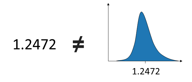
Fig. 2: Example of back transformed values at a single location.
If we back transform the estimated Gaussian mean as if it’s a single number, the result is some kind of franken-mean that, at best, approximates the true mean at the estimated location (red; Fig. 2). It is theoretically invalid to do this. Instead, the Gaussian distribution must be fully back transformed, usually by discretizing it by a large number of randomly or equally spaced quantiles, back transforming those quantiles using the constructed lookup table from forward NS transform, resulting in the blue distribution in Fig. 2. Then, meaningful statistics can be calculated from this distribution (black; Fig. 2).
The Takeaway
MGK is an extremely powerful tool to assess uncertainty. However, the estimate must be treated appropriately since it is not a single value, but a distribution which can provide many other measures that may be of interest, e.g., probability to be within +- 15% of the mean, probability to be above a certain cutoff, etc.
Resources
- MultiGaussian kriging for grade domaining. 2012. SRK. https://www.na.srk.com/en/newsletter/mineral-resource-estimation/multigaussian-kriging-grade-domaining-uncertainty-based
- Leuangthong, Oy, and R Mohan Srivastava. On the Use of MultiGaussian Kriging for Grade Domaining in Mineral Resource Characterization. In Ninth International Geostatistics Congress. Oslo, 2012.
- Babak, Olena, and C. V. Deutsch. Testing for the Multivariate Gaussian Distribution of Spatially Correlated Data. CCG Annual Report 10. Edmonton, AB: University of Alberta, 2008. http://www.ccgalberta.com.