The Experimental Variogram: Can’t Live With It, Can’t Live Without It...
TL;DR
Each point of an experimental variogram represents the spatial correlation between a set of data pairs that are separated by a particular distance and direction. As you increase the distance between pairs of data along the same direction, AKA move to the next lag distance, spatial correlation decreases (not always… yes, I know, you TROLL!). The variogram ($\gamma(\mathbf{h})$) is related to spatial covariance ($\mathbf{C}(\mathbf{h})$) through the stationary variance ($\sigma^2$):
$$ \gamma(\mathbf{h}) = \sigma^2 - \mathbf{C}(\mathbf{h}) $$
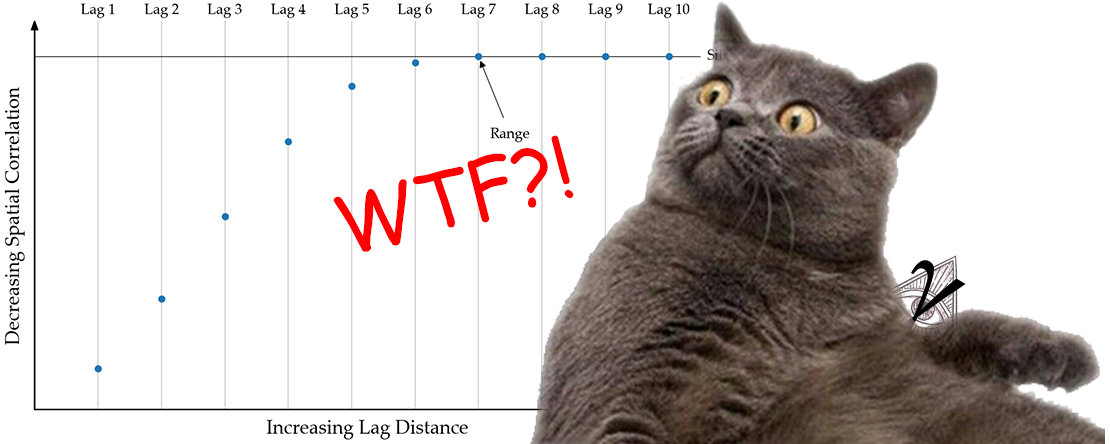
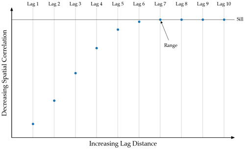
As spatial correlation decreases with increasing lag distance ($\mathbf{h}$), the variogram points approach the sill (the variance of the data $\sigma^2$), at which point pairs of data at that distance (the range) and beyond are not correlated.
You calculate the experimental variogram using each set of data pairs along a specific direction for all of the different lag distances. Once you’ve collected all data falling into each lag distance “bin,” you can use a variety of algorithms (covered in a future post) to calculate the variogram value for that lag.
Spatial Correlation!?
Correlation is typically thought of as the relationship between two variables measured at a single observation. However, two composites within a deposit separated by some distance can also be correlated (spatial correlation). For the geological minds out there, I’m going to lay out a straightforward thought experiment. Think of a deposit with geometry that isn’t that complicated, something like an unaltered Fe-Ti-Vi cumulative deposit that hasn’t been structurally complicated. The main geological process in this setting is fractional crystallization, forming layers of titanium-vanadium-rich magnetite in the upper parts of layered mafic-ultramafic intrusive complexes over time. So, if you were to drill a vertical hole and collect a sample, it is reasonable to expect the metal concentration of the rock 20 metres away laterally would be very similar to that sample. While the rock 20 m downhole is less likely to be as similar. In other words, two samples collected increasingly farther away from each other at the same elevation (same horizontal layer) would remain correlated for quite some distance. Conversely, as you increase the distance between two samples from the same drillhole, the maximum distance they remain correlated will be much less than the samples collected from the same elevation.
FYI, I use spatial correlation and spatial covariance interchangeably, but technically, spatial correlation is just the standardized spatial covariance. You can convert between the two as follows:
$$ \rho(\mathbf{h}) = \mathbf{C}(\mathbf{h})/\sigma^2$$
The Components of an Experimental Variogram
The experimental variogram is the representation of the interrelationship of a property between two locations that are separated by some distance in some direction. Each point on the variogram plot represents the spatial correlation between a set of data pairs, and each pair is separated by a specific distance called “lag distance.” Together, these points capture how the spatial correlation of a variable changes with distance. Eventually, pairs of data will not be correlated with each other. The switch from correlated to not correlated happens at a distance imaginatively called “the range." We can tell that data is not correlated at the range because the experimental variogram reaches the “sill,” which is equal to the variance of the data. The figure below illustrates all the components of an experimental variogram.
How Is It Calculated?
Before I get started, you typically calculate experimental variograms in three directions. I’m going to expand on that in a future post where I talk about experimental variogram calculation parameters. Also, there are a few different algorithms that can be used to calculate the variogram value at each lag (e.g., correlogram, pairwise relative, etc.) that i’ll cover in another post.
The magic to calculating an experimental variogram is to generate all the sets of data pairs used to calculate each lag distance point. Imagine visiting the centroid of a composite then calculating the direction and length of all of the vectors that separate it from all the other composite centroids. When calculating the experimental variogram for a single direction at a specific lag distance, all the composite pairs that are separated by a vector matching that direction and distance get paired together. And when I say paired, I mean the composite’s metal value at your current location (the tail) is matched up with the metal value of the other composite (the head).
Below is an animation that shows a simple 2D case that evaluates all lags used to define the experimental variogram. The top left image illustrates the set of data pairs found for each lag distance. The head and tail data of each pair are red if their separating vector (black line) has an azimuth between 0 and 24 and a distance +/- 5 metres of the specified lag distance in the title. The scatter plot in the top right (h-scatterplot) illustrates the correlation coefficient ($\rho$) between the head and tail values. The variogram plot on the bottom shows the experimental variogram value calculated using each lag distance’s set of data pairs. You can see that as the correlation coefficient decreases for each subsequent lag in the h-scatterplot, the variogram value moves closer to the sill. Once the variogram intersects the sill, the correlation is zero. Variogram values above the sill are negatively correlated.
Why Do I Need to Care?
We calculate the experimental variogram using our data, but they are limited as they only illustrate spatial correlation in specific directions. We can calculate the expected spatial correlation between two points at all distances and directions using a variogram model that is fit to the experimental points.
When Kriging is estimating a block, it uses the variogram model parameters you give it to determine which composites within a search ellipsoid are spatially correlated with each block. The algorithm calculates a weight for the correlated composites; otherwise, they receive a weight of zero if the distance between the block and composite is larger than the variogram range.
Additional Readings and References
- Rossi, M. E., & Deutsch, C. V. (2014). Mineral Resource Estimation. Edmonton AB: Springer Netherlands. https://doi.org/10.1007/978-1-4020-5717-5
- Ed Issaks videos on YouTube
- Michael Pyrcz videos on YouTube
- Geostatistics Lessons on Variograms
- The Practical Geostatistics series
- Gringarten, E., & Deutsch, C. V. (2001). Teacher’s Aide Variogram Interpretation and Modeling. Mathematical Geology, 33(4), 507–534. https://doi.org/10.1023/A:1011093014141