Transformations

TL;DR

This post is the start of a series on common data transformations in geostatistics, where we apply them, and why we apply them. We need transformations because real data is … complicated, especially in geological environments. There are a wealth of data transformations we can apply. Some are one-directional (capping), some change distributions to appease modeling assumptions (normal scores), some treat our biased spatial sampling (declustering), and others change how we look at the data to reveal other relationships (embedding or dimensionality reduction).

Introduction

There are a wide variety of transformations that can be applied to ‘data’ (see the sklearn API for an example).

A ‘transformation’ in this context takes a set of values, and changes those values for a specific purpose. Transformations may or may not change the shape of the data. The set listed above are machine learning (ML) oriented, and are mostly concerned with regularization - that is, taking a set of inputs, with vastly different ranges or representations, and putting them all on the same ‘level’ so that various ML algorithms will extract meaningful things. The transformation pipeline is arguably the key to ML success.

In geostatistics, transformations are also a major contributor to success; we have specific problems that require specific treatments:

• Extreme Values
• Detection Limits
• Spatially Biased Sampling Patterns
• Distribution Assumptions in Modeling Algorithms
• Compositional Data (whole rock, grain size distributions)
• Linearly Correlated Multivariate Data
• Non-Linearly Related Multivariate Data
• Non-Stationary Spatial Relationships
• And Others …

Not surprisingly, there are a wide range of transformations developed to address each issue in a range of different domains. In this post we’ll examine the first 3 on the list: capping for extreme values, despiking for detection limits, and declustering to treat biased sampling.

Capping Extreme Values

Capping comes down to management of outliers. Capping is most important for highly skewed grade distributions (Au, Ag, …), where extreme values can have a significant impact on the generated models. Choosing a capping value is non-trivial; there are no deposit-agnostic rules to follow only some good guidelines. Assuming the deposit has been mined the best bet is to calibrate against production data and with reconciliation. Given you have determined a cap value, the cap-transform simply finds values above or below your min and max, and resets to the chosen capped min/max. Simple. But, why?

Capping comes down to limiting the ability of outliers to influence unreasonably large volumes given the known continuity and the support of the sampling. Consider this vein example (all credit to original post!):

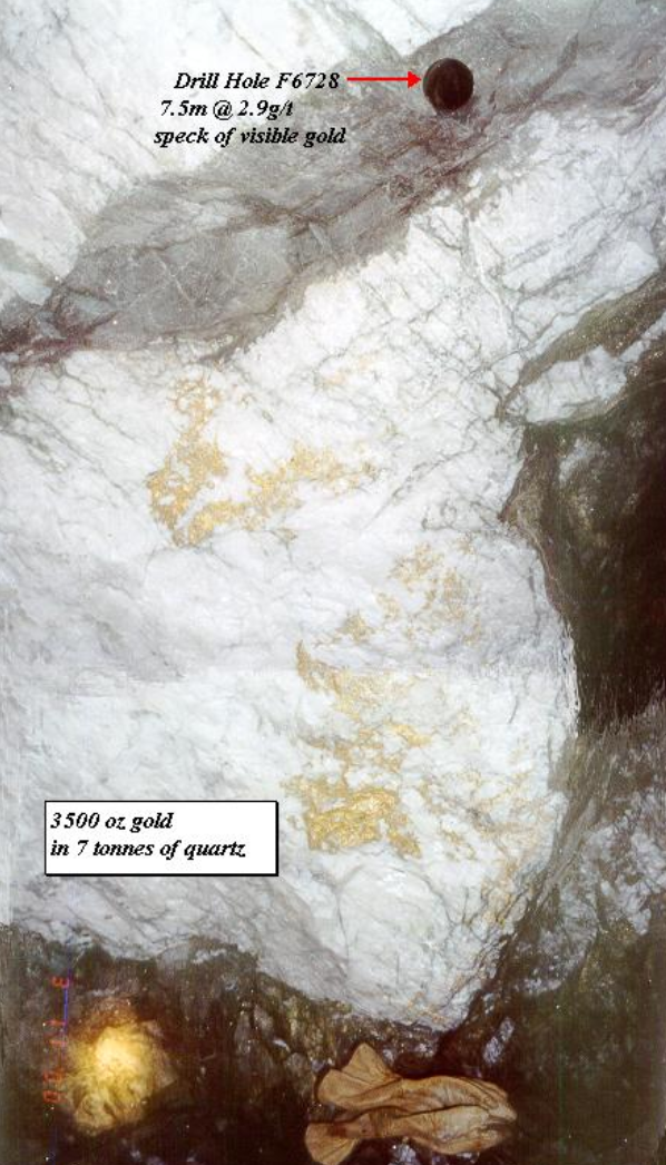
Imagine the drill hole from this example intersected the vein in an exploration campaign. Without additional nearby sampling, or an understanding of how common such intersections would be, the extreme value could influence a much larger area than is reasonable (shudders…).

Despiking Detection Limits

Spikes only need treatment in Gaussian transformations. A ‘spike’ simply refers to duplicate values in a given dataset. Not duplicate locations (another problem we’ve got to deal with!), but duplicate assay values, like 0.001 occurring all over the place. All geochemical analyses have lower and upper bounds (detection limits), and carry a certain amount of significant figures. Consider the following gold (Au) assays:

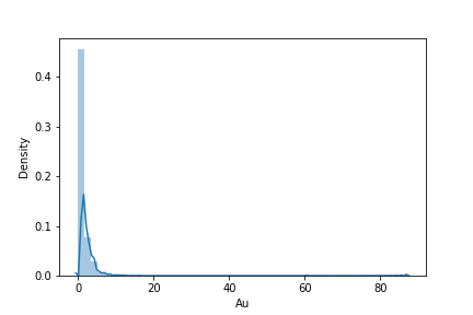
Which has a minimum of 0.01, max of 87.. Nothing seems wrong so far… Transforming these values directly to be Gaussian with a Quantile-Quantile (QQ) transformation:

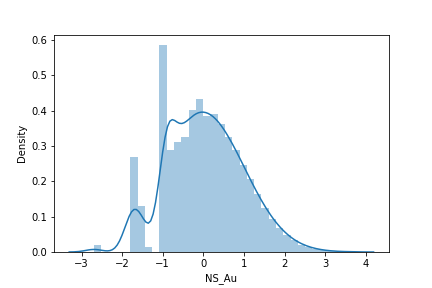
Yikes! This is not a nice looking Gaussian distribution. In terms of correctness, the shape is incorrect, the mean is 0.03 (close to 0.0, but not perfect… acceptable?), but the variance is 0.89, which is fairly off of the target 1.0. Looking at the frequency of values occurring in the dataset (kind of like a histogram… but without bins):

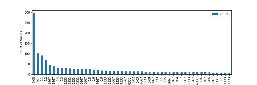
And look at that.. The most frequent values are 0.05, 0.01, 0.1, 0.2 and so on… Each of those is getting transformed to a single Gaussian value, which is making our final Gaussian distribution look not so Gaussian.

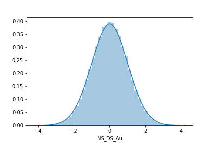
Despiking applies a small random number to the spikes so that the result of transformation looks more Gaussian.. like this:

The only thing we’ve got to consider is what kind of despiking to apply… or, should we even despike at all?

Well, if we’re targeting Gaussian geostatistics, then yes, despike. Conditional simulation and multiGaussian kriging strictly assume the distribution is standard normal, so failing to meet that assumption is likely to give unexpected results. However, if we’re targeting some ML algorithm with the transformed values, then we should possibly forget the despiking step and instead preserve those spikes. Consider below; if we despike prior to Gaussian transformation, we end up with values that are equal in original units (y-axis), and spread them out over a range of Gaussian values (x-axis):

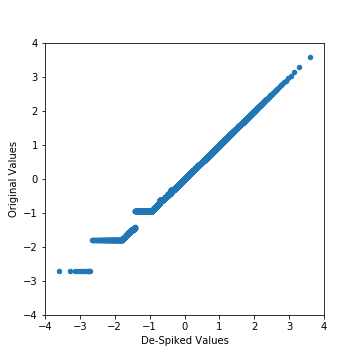
In ML algorithms, this implies that originally equal values are no longer equal, which means that there is a gradient that decisions can be made on… But, this is entirely artificial since we introduced the difference with a random value added to our original data… So, probably skip despiking in this case!

Declustering Biased Sampling

Clustered sampling is the norm in geological datasets since areas of high value are (of course) preferentially sampled to quantify extents as best as possible. However, calculating statistics from the raw dataset and drawing conclusions from those statistics without any kind of treatment to the sampling configuration within some reasonable domain extents should be raising all kinds of red flags.

Aside: "high value" might be indicated by highs (like Au grades) or lows (like vshale in oil and gas)

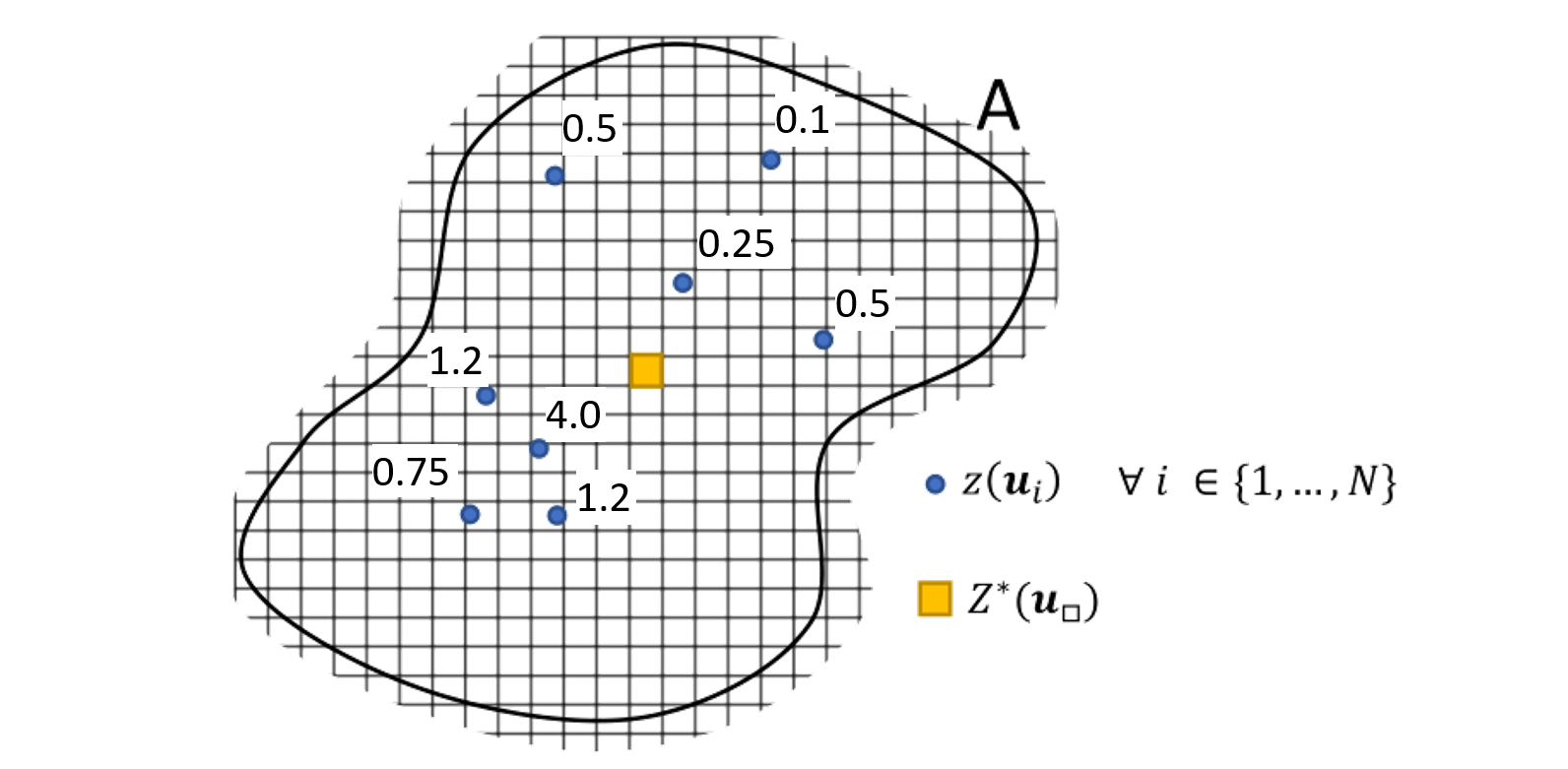
Declustering is applied in nearly all geostatistical modeling workflows. Declustering is the process of calculating weights for each sample location proportional to the area (or volume) that the sample represents. For example, below, a schematic of a fictional domain A shows the total domain boundaries (dark line), 4 tightly-spaced samples in the bottom left and 4 sparser samples in the top right, with the grade values labeled at each location. Since the samples from the top are more equally spread out, each will be assigned more weight since each is less redundant. By contrast those in the bottom left are closer together, more redundant and will be assigned more variable weights based on their position.

Declustering doesn’t actually change the value of the samples, instead it changes how the samples contribute to the statistics calculated within specific volumes. In this sense we’re transforming our distribution from clustered to representative. For example, let’s say the top four samples get equal weight. The bottom four samples have higher grade intersections but … are more redundant, particularly that 4.0 sample in the middle. The CDFs of the un weighted (blue) and weighted (orange) cases for this scenario are shown below:

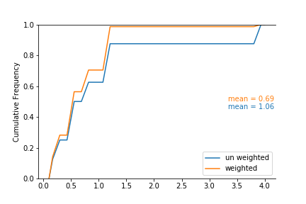
Recalling our CDF interpretation skills, large vertical jumps indicate a high proportion of that value in the distribution. In the un-weighted case, there is a large vertical jump around 1.2 and 4, which happens to coincide with the 2 samples of 1.2, and 1 sample of 4.0 equally contributing to the global distribution. However, when we apply our declustering weights, the contribution of the 1.2’s is slightly increased, and the contribution of the 4.0 is majorly decreased, which overall results in a significant decrease in the global mean in this toy domain. Declustering, in practice, might make for a sad story in some environments, but it’s realistic and fair; we can’t allow our global statistics to be equally influenced by all data unless that is warranted.

Final Thoughts

Geological data and geological data problems will always have a special place in my heart. Mostly it’s how you want to use the data that makes problems, and depending on your toolset these problems can either be a joy or pain to deal with. But like it or not, we need transformations to facilitate all the workflows.