Conditioning... What? And a Small Rant about Jargon
TL:DR
Conditioning relates to the probability of one event given another related event has occurred. Probability distributions may be conditional to related nearby observations, and ultimately this translates to a reduction of uncertainty by incorporating observations to predict related events.
Introduction
Starting out in any scientific field is challenging. Jargon is one of the many hurdles. Experts need to ‘speak the same language’ and represent complex ideas in simplified terms. Fine. But before you know this language, things are confusing! This post breaks down the concept of ‘conditioning’ (and all related verbs, adjectives, nouns). Nearly 6 weeks into my studies at the U of A I scribbled ‘WTF is conditioning’ out of pure confusion (see image above). That first semester with ‘conditional’, ‘conditioning’, ‘condition’ terminology flying around (among others), it was just pure chaos trying to understand what I was being taught.
The actual meaning of ‘condition’ is not difficult, but if you don’t have the background or don’t understand the context, it can be challenging to understand all the ways this terminology is used. So, let’s dive in and attempt to understand this important statistical concept!
Probability
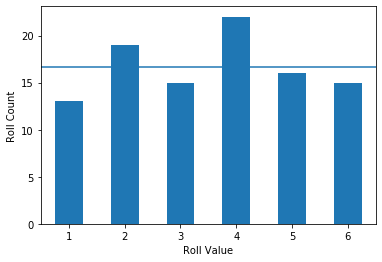
Let’s quickly recall probability: given some number of observations from a system we can quantify the probability of specific outcomes. The probability of all possible events is summarized by a probability density function (PDF); a simple example of this is repeated dice rolls. Let’s say we take 100 rolls as our sample. A PDF of the sample is shown below. The horizontal line shows the theoretical probability of each event ($ \frac{1}{6} $).
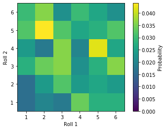
Real systems commonly have many variables which may be related in interesting ways. In the case of multiple die, each roll is independent. Rolling one tells you nothing about the next one. Inspecting a bivariate PDF (below) of 500 repeated rolls shows fairly random relationships (no linear features here), and if we repeated this experiment infinity times each bin should contain the theoretical $\frac{1}{36}$ probability:
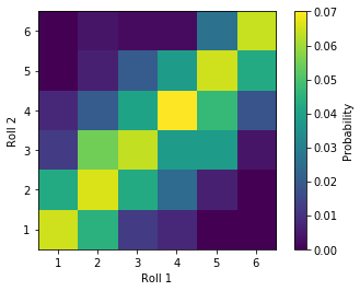
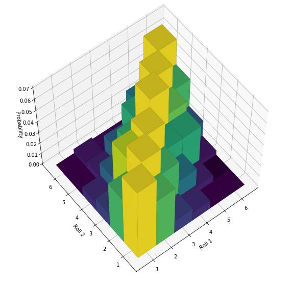
Imagine we have trick dice that are highly likely to roll the same value, in other words the outcomes of their rolls are strongly correlated. Given we know the value of the first roll, we can make a pretty accurate guess on the value of the second. This property of the trick dice rolls is summarized in the bivariate PDF below; we see a linear feature going along the main diagonal, which tells us that the rolls of the dice are likely to be similar, atleast much more so than rolling ‘regular’ dice above.
Sometimes looking at these bivariate PDF’s in 3D helps. Below the linear ridge of ‘high probability’ is shown with vertical bars:
Conditional Probability
The terminology ‘condition’ (and all related verbs, adjectives, nouns) in this context relates to the effect of the first roll on the outcome of the second. The second event is referred to as ‘conditional to’ the first. Conditional probability formalizes this to calculating probability in the presence of related events. In equation form this is described by:
$$ P\left( A | B \right) = \frac{P\left( A & B \right)} {P\left(B\right)} $$
Which reads literally as the probability of event A given (conditional to) event B equals the probability of event A and B (joint) divided by the probability of event B (conditioning event).
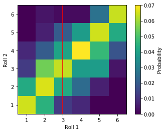
Relating to the dice example, we have observed enough trick dice rolls to generate the bivariate PDF above. Therefore, we know the joint probability, since we have counted how many times (over a reasonable sample size) we got each combination of roll results. If we know that Roll 1 is a 3, we take the joint probability of ~0.061 and divide by the probability of the first roll resulting in 3 (~0.16), which results in a probability of 0.375 or a 37.5% chance to roll a 3. Compare this to the true independent case, the probability of 3 from the second roll given the first is $\frac{1}{36} \div \frac{1}{6} \approx0.16$, or the same probability as if the conditioning event never happened!
There! That is the basic essence of ‘condition’. Observations of related events are used to constrain distributions where we have no information. In a geostatistical context the samples become like the Roll 1s and all the unsampled locations are the Roll 2. Samples are used to improve the estimates at the unsampled locations through conditioning.
Conditional Distribution
Looking back at the bivariate PDF of our example of trick die (colored squares), the first roll becomes the conditioning event (red line), which conditions the distribution of possible values that may be observed from the second event:
Conditioning Data
Conditioning data are observations (e.g., drillhole composites) used to generate estimated distributions where we have no observations (e.g., blocks in a model). We call the data within some domain the ‘conditioning data’, because those data will be used to condition the distributions at the unsampled locations, e.g., constrain the distribution both in terms of mean and variance in accordance to the relationship between locations as defined by the variogram and the values of the conditioning data).
Conditioning Effect
This is the one that had me scratching my head during my lecture at the U of A, e.g.:

The discussion was with respect to mean uncertainty, the bootstrap, and the spatial bootstrap, and how conditioning data with spatial correlation affects how random samples should be drawn from a domain. Note: This is quickly getting beyond the scope of conditioning and is using jargon to explain jargon… we can’t escape it…
Aside: the bootstrap is a method to calculate uncertainty in the mean by resampling the input histogram many times and calculating the mean of the resampled values.
The outcome of bootstrap and spatial bootstrap can be very different because of conditioning, where locations inform possible values at other locations since they are spatially correlated. Essentially the spatial correlation makes all samples more redundant, which ultimately results in more uncertainty. This is definitely getting beyond the scope of this discussion, but conditioning forms the basis of this thought train and is an important concept in geostatistics. This all relates back to the fact that every location is a ‘variable’.. I find this figure from Jeff Boisvert’s PhD Thesis particularly helpful to visualize this:
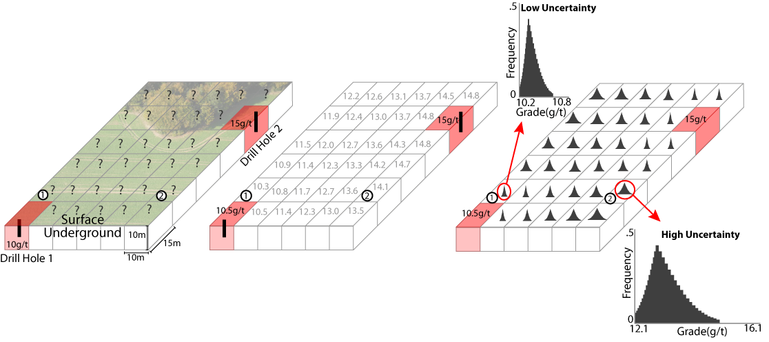
Looking at the above left figure, we have 2 samples (red) and many unsampled locations (?’s). The two samples are the conditioning data. Looking at the right figure, we see that there are distributions of possible values at each location where we don’t have a sample. These are the conditional distributions generated through kriging, simulation or other means.
Other Conditioning terminology
Thought I’d just throw a list of other things related to conditioning that may possibly be explored in future posts:
- Conditional Bias
- Conditional and Unconditional Realizations
- Conditional Covariance
- Uniform Conditioning
- …
Final Thoughts
Conditional probability is the fuel of geostatistics - we use observations collected from a domain to condition distributions of uncertainty where we don’t have any observations. Conditioning reduces the uncertainty at the unsampled locations. Conditional distributions are generated with nearby related data, where the relationship is dictated by the spatial correlation derived from the variogram.