WTF is that Equation? The Variogram

For today’s episode, we are going to dive deep into the equation used to calculate your experimental variogram. So break out your nerd hat and hang on for the ride. Don’t worry though, we’ll be trying to take as much of the WTF out of the equations as we can. Despite diving deep, I’ll be trying to keep things pretty shallow which means that I’ll gloss over a lot of the fine print that most people don’t read anyways, but that do have a habit of coming back to bite you in the ass when you least expect it. So be for-warned. Also for this post, unfortunately, there is no TL;DR because the TL;DR is the equation. 🤷

Graphs and spatial structures:

Ok, before I dive into the nuts and bolts of the equations let’s set the story a little bit. First off, having a general sense of what a variogram is will be helpful. So, if you are feeling a little unsure I’d jump on over to our previous posts on the experimental variogram. Calculating the experimental variogram, and other measures of spatial structure, like the correlogram, is all about figuring out the spatial correlation in your dataset. Most of us are doing this for a single variable at a time, but this can be done between as many variables as you want, depending on how masochistic you are feeling.

Recap of the Semi-Variogram

Let’s step back a little further. Most of us have seen a variogram such as this, though only in textbooks and probably never one this nice in real life! In fact the only way I found one this nice was by stealing from our previous post

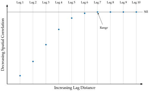
So what is a semi-variogram? It’s a graph (or -gram!) in which the semi-variance is plotted on one axis (the ordinate or y-axis) against some “distance classes” on the other axes (the abscissa or x-axis). These “distance classes” are often just talked about as “lag” distances. So a lag of 10 meters means that you are calculating the semi-variance between all pairs of data that are spaced every 10 meters. That seems pretty easy, let’s break out that equation then! Side note Most people, like us, are lazy and get really tired of calling it the semi-variogram, I mean that is an extra syllable! and no one really calls it the graph of the semi-variance, that’s way too many syllables! So we all just shorten things and call it the variogram.

Breaking apart the equation

$$ \gamma(\mathbf{h})= \frac{1}{2n} \sum[Z(\mathbf{u})-Z(\mathbf{u}+\mathbf{h})]^2 $$

Now like all good scientist, let’s break up this equation and define our terms

• $ \gamma $ = Semi-Variogram
  • Side-Note: Historically, the 2 was often moved to the left side of the equation for mathematical convenience. So $2 \gamma $ is the “variogram” versus $ \gamma $ being the semi-variogram which is half of the variogram
• h = distance vector (aka the lag distance).
  • What does this mean? Well, we are going around finding what the semi-variogram is at a specific distance and vector. So $ \gamma $(10) means we are going around and visiting every value and looking at what values are 10 units (ft, m, etc) away.
  • The vector would include distance, and direction (strike and dip)
• Z(u) = The available data of variable Z at location u. (Most books will say: realization of the random variable Z at location u)
  • Yeah, that’s a mouthful. Fancy way of saying the variable of interest at the location u. If we are calculating the variogram for Au, then Au(u) is the value of gold at location u. Because we are dealing with spatial data, that sample has some spatial coordinate associated with it.
• [Z(u) - Z(u + h)] = pair of data at distance/vector h
  • For each distance vector, we are finding all pairs of data. So if we are looking at Au with a lag distance of 10 meters, we are going around and finding all of the Au samples in our dataset that are 10 meters apart (usually looking in a specific direction)
  • It is sometimes helpful to distinguish between the points in the pairs. So as we go around finding the pairs, we go to a location Z(u), this is the “tail” and find another data point Z(u + h) at h distance/vector away, which becomes the “head”
• n = the number of pairs we’ve found at the distance vector we are calculating.

Semi-Variance

So, the variogram is the expected squared difference between all pairs of data values that are at a specific distance vector away. Now that we’ve explained our terms, let’s take a quick step back. Does our semi-variogram equation almost look familiar? How about this equation?

$$ \sigma^2 = \frac{1}{n} \sum(x_{i} - \bar{x})^2$$

Yep, that’s your ol’ trusty equation for the variance of a dataset. As we said above, the semi-variogram is just a plot of the semi-variance for a set of lag distances. The variance looks at the squared difference from the mean, while the semi-variance (spatially) is half the squared difference of the data points h distance/vectors apart.

Now that we have a general understanding of what the semi-variogram is and our terms, let’s go through the calculations step by step.

Uniform Example

For our example we’ll stick with 2D and we’ll say we are calculating the variogram at 2 units away directly to the east. How does this work out? First we loop through every sample in our Au database. Then at each sample location we say we are at u. From u, we look around us in the “h” vector. 2 units in the East direction.

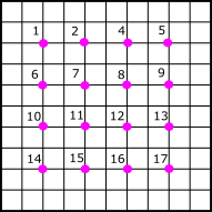
So with the above example, at sample location 1 we search to the east and find sample 2. Similarly, sample 2 is paired with 3 and so forth and so forth. Next we decide to look at a lag distance of 4 units to the east. So yep, that means as we are looping through sample 1 is now paired with sample 4, and if we jump ahead we would see that sample 15 would be paired with sample 17 and so forth.

More Complex Example

There is one problem with the above example.. Most often our data are not sampled on a perfect grid; how often will samples be exactly 4 units away?!? What if it’s 4.05 units away? Therefore most software includes tolerances in the variogram calculation. So let’s look at a slightly more realistic 2D example.

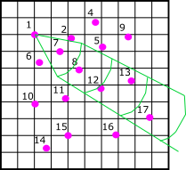
Now we have a variety of spacing in our drilling, and we are interested in looking in a more unique direction. We’d set up the direction we are looking in and we’d set up some tolerances. So I’ve drawn an example of some tolerance and different lag distances in green lines above centered on our sample 1. Now our first lag distance sample 1 is paired with sample 7. For our third lag, sample 1 is paired with sample 12 and again sample 1 is paired with sample 13 (because of the tolerances sample 1 is being paired with 2 different samples in this lag.

So let’s recap a little about how this works.

1. First we loop through every sample in our Au database.
2. At sample (u), we look around us in the “h” vector (say 8-12 meters away between 40-50 degrees).
3. If we find another sample within our “h” vector bin, then we calculate the squared difference between our pairs, and increase our pair count by 1.
4. We do this until we find all pairs of data within our “h” vector.
5. Now we divide by our total number of pairs to get the semi-variogram for “h” vector
6. Repeat steps 1-5 for each one of our lag distances

And there you have it! That is how to calculate your variogram in a nutshell. 🌰

Extra resources:

I did gloss over a lot. So, if you want to dive deeper, here are some extra resources you might be interested in checking out.

• For a good indepth discussion on the variogram parameters such as setting up your tolerances, check out the geostatistics lesson on it here
• If you want to step through some more concrete examples and see the actual calculations
  • Edward Issaks has a nice video over on youtube. Check him out here.
  • Michael Pyrcz also has one of his lectures online with a fairly detailed video here, you just have to forgive him for his use of the Jet colormap.
• We are also building up a good collection of topics around the variogram which you can check out here
• If you are wanting a more textbook approach, I’d suggest The Practical geostatistics series. The older version is free and well written.