The Correlogram & The Third String Backups
TL;DR
Once you’ve collected all the pairs of data that fall into each lag distance “bin,” you can use various algorithms to calculate the experimental variogram value for that lag. Each has its pros and cons.
The traditional variogram is very sensitive to issues with the data (e.g., outliers, proportional effect, etc.), but it can work in some situations. The correlogram is a robust alternative that handles precious metals well. The covariance algorithm is very similar to the correlogram, but I tend to use the correlogram anyway. Using the traditional variogram algorithm on data that has been normal scored, which cleans up your data, can produce a better behaved experimental variogram. But, be sure to back-transform the variogram model you fit using normal scored data correctly if you’re using it to model a variable in original units! And finally, the pairwise relative variogram can be very good at dealing with a tricky dataset that the other algorithms find too hot to handle. However, be careful when using a pairwise variogram. Not all software is programmed correctly, so it may not be used right, even though they offer it.
Introduction
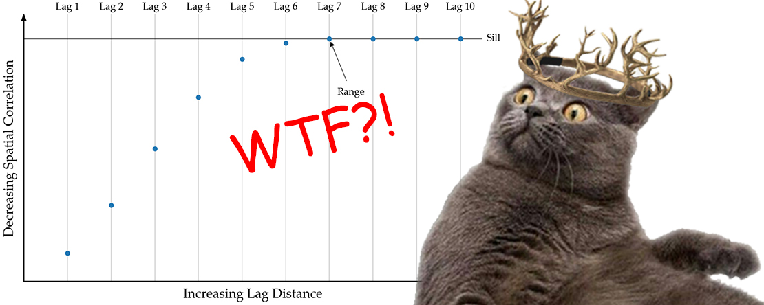
This post is a continuation of the “WTF is a Variogram Series.” So if you haven’t checked out the previous post on what a variogram is or what an experimental variogram is, be sure to check them out before giving this a read. If you already have, well… who’s better than you?! No one, obviously.
So we (and by “we” I mean “you”) went around and collected a bunch of pairs that are separated by a specific distance and direction, each bunch falling into a lag distance “bin.” Now we need to use each lags bunch of pairs to calculate a single variogram value that we can plot up and fit a variogram model too! To do that, you can pick from a bunch of different “algorithms.” The most popular algorithms include the one-and-only traditional semi-variogram, the correlogram, the non-ergodic (🤓) covariance, the often misused and abused normal score variogram, and the black-sheep pairwise relative variogram.
Algorithms to Calculate the Experimental Variogram
Traditional Variogram
The OG algorithm… actually, it’s more like the King Joffrey of variograms, crazy as hell and impossible to control. It averages all the squared differences (mean squared error) of all pairs found in each lag “bin.” When calculating the mean squared error, outliers, crap data, the proportional effect, and/or high variability can REALLY make your experimental variogram noisy. Some variables such as gold will not play nice with this algorithm, and you’ll be pulling out what little hair you have left, if you have any at all.
Correlogram
The One True King of variogram algorithms! It’s great to use when you’re dealing with a variable in original units that has some proportional effect issues, AKA gold and other precious metals. It considers both the distance between sample pairs and the local means of the head and tail values. Meaning for each set of data pairs, it grabs all the head values and calculates their mean and grabs all the tail values and calculates their mean. In fancy geostatistics words, it is more of a non-stationary flavour of an algorithm than its rivals as it considers the local mean and variance of the head and tail values. And by non-stationarity, I mean there are various trends in the data, shifts from high to low grades and everything in between.
Non-Ergodic (Non-Stationary) Covariance
If you don’t know what non-ergodic is, don’t worry about it. Knowing so won’t bring any more joy to your life, just think non-stationary. This algorithm is the less famous cousin of the correlogram as both are a non-stationary flavour. The non-ergodic covariance considers the mean of the head and tail values and doesn’t assume they are the same, but it does not consider their variance, unlike the correlogram. In practice, I’ve found it to perform better than the traditional variogram, but tend to end up using the correlogram as it tends to behave better.
Normal Score Variogram (NS Variogram)
If you’ve transformed your data into a Gaussian distribution and calculate the experimental variogram with the semi-variogram algorithm, you’re calculating an NS Variogram. While not actually a new algorithm, transforming the data into a Gaussian distribution gets rid of that pesky proportional effect and helps handle outliers, both things that make calculating the experimental variogram easier.
❤️ PUBLIC SERVICE ANNOUNCEMENT ❤️
PLEASE FOR THE LOVE OF GOD DO NOT TAKE THE VARIOGRAM MODEL PARAMETERS THAT YOU GOT USING TRANSFORMED DATA AND USE IT AS INPUT TO ESTIMATION OR ANYTHING ELSE WERE YOU ARE USING THE VARIABLE IN ORIGINAL UNITS!!!
YOU NEED TO BACK TRANSFORM THE VARIOGRAM IN A VERY SPECIAL WAY!!! THEN GET THE PARAMETERS OF THE BACK TRANSFORMED VARIOGRAM.
OK!!?!
THERE IS A GEOSTAT LESSON ON IT HERE!
❤️ THANK YOU ❤️
Pairwise Relative Variogram
This algorithm would be the oddball/outcast of the variogram algorithm boy band if that ill-conceived idea becomes a reality. It’s great when dealing with sparse, clustered, and/or erratic data… but its sill isn’t the data’s variance, making it the unique little snowflake it is. Seriously use caution when using this in various commercial software. Two very popular mining suites cannot tell me how they calculate the sill when selecting this variogram algorithm… Which doesn’t instill a lot of confidence. It is possible to calculate the sill transforming the data to a log distribution (Babakhani and Deutsch 2012) or simulating it. I sometimes use it to confirm the ranges I see in my experimental variogram calculated with a different algorithm. When I do this, I try to approximate where the sill would be in my head; in most cases, you’ll see the points flatten out below the data’s variance. Oh, and make sure your data is all positive (not emotionally, I mean their metal values) if you use this bad boy.
Additional Readings and References
- Rossi, M. E., & Deutsch, C. V. (2014). Mineral Resource Estimation. Edmonton AB: Springer Netherlands. https://doi.org/10.1007/978-1-4020-5717-5
- Ed Issaks videos on YouTube
- Michael Pyrcz videos on YouTube
- Geostatistics Lessons on Variograms
- The Practical Geostatistics series
- Gringarten, E., & Deutsch, C. V. (2001). Teacher’s Aide Variogram Interpretation and Modeling. Mathematical Geology, 33(4), 507–534. https://doi.org/10.1023/A:1011093014141
- Wilde, B and Deutsch, C.V., (2006). Robust Alternatives to the Traditional Variogram. CCG Annual Report Paper
- Babakhani, M and Deutsch C.V. (2012). Standardized pairwise relative variogram as a robust estimator of spatial structure. CCG Annual Report Paper