These kriging weights are really, really ridiculously good looking...

TL;DR

In the realm of estimators there are many ways to determine the weights applied to our nearby samples to estimate the value at any specific location. Nearest neighbor (NN) and inverse distance squared (ID2) weighting both only use the distance from the sample to the estimation location to calculate the weights. Kriging and Radial Basis Functions (RBF) account for both distance from sample to estimation location and the position of the samples in relation to each other. By also taking into account the relative position to other samples, Kriging and RBF’s sometimes give rise to the sometimes perplexing but still logical negative weights…

Jupyter notebooks associated with this post can be found here and here.

Introduction

Following the implementation of custom estimators in Python, we’ll look at how NN, ID, Kriging, and RBFs weigh nearby data when calculating an estimate. Some of the results are interesting and expected, but perhaps not immediately logical. Using some simplified 2D and 1D examples, I hope to illustrate the differences between the methods and why they exist. That way, you can have a deeper understanding of what is going on under the hood and know which estimation strategy is best for your project.

Test Data

We’ll focus on two cases, both subsets of the example domain from last time. Both cases are simplified to 2D to permit easy interpretation of the location’s relationship to weights (e.g., there is no hidden data into or out of the page!).

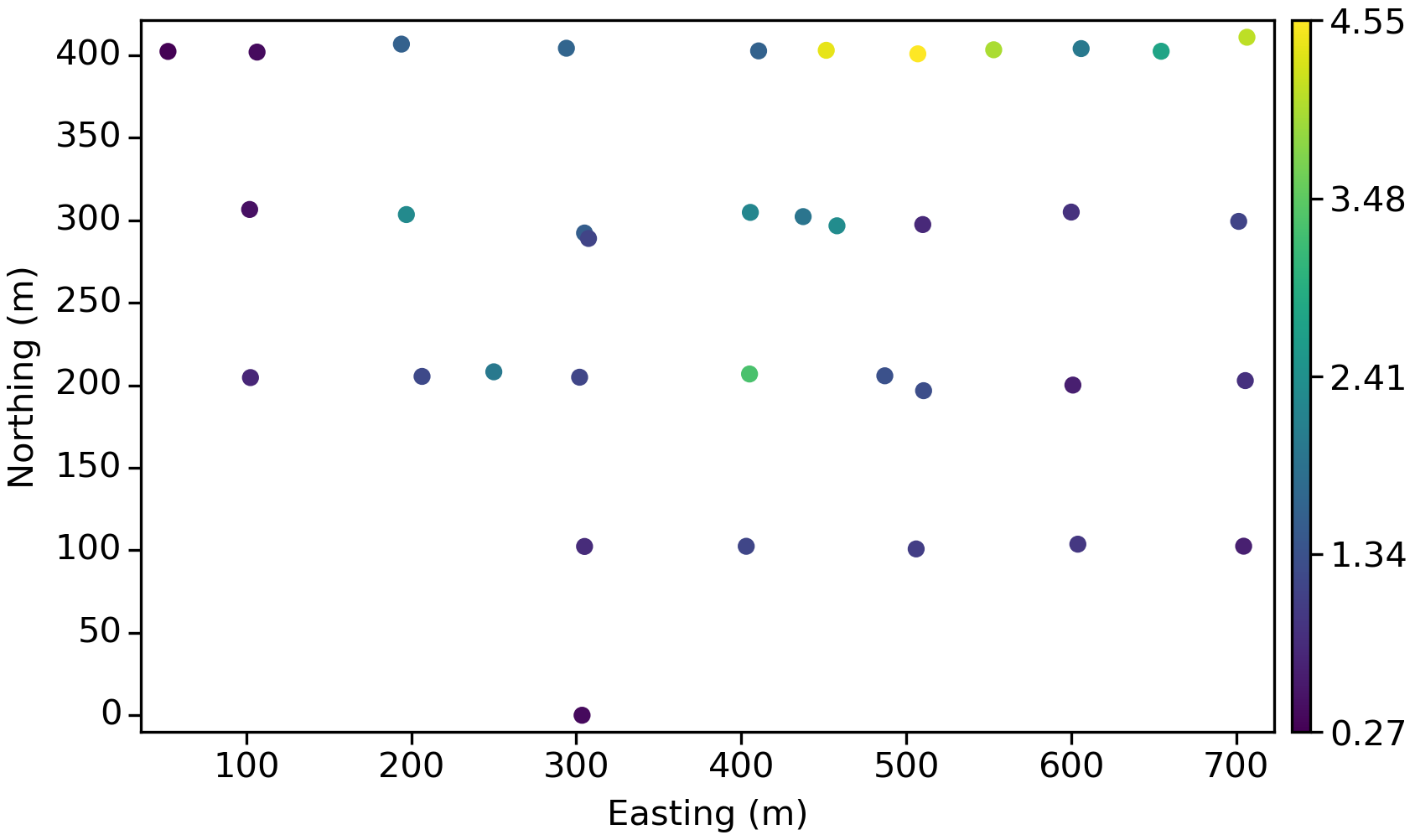
The first case takes a plan-view slice through the data, for an overall equally-spaced collection of samples shown below:

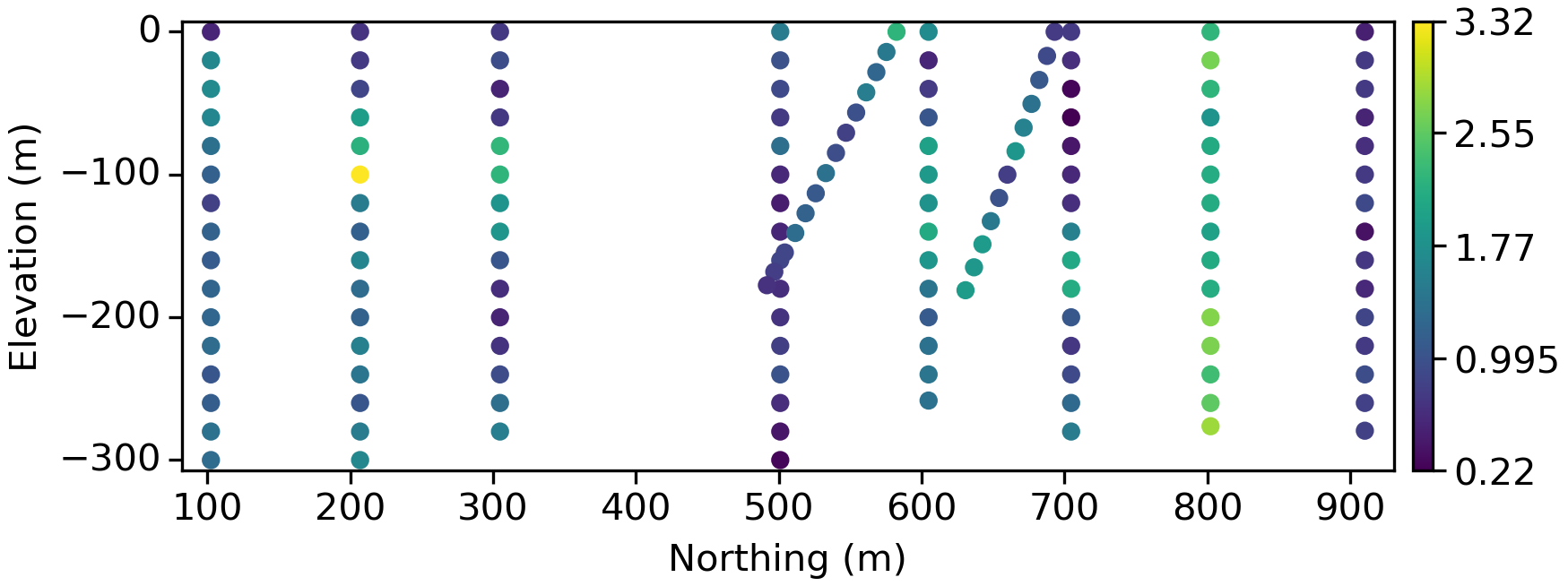
The second configuration is a vertical slice through the dataset along a single fence and captures one of the “fun” properties of drill data, where the sample spacing down hole is often much smaller than between holes:

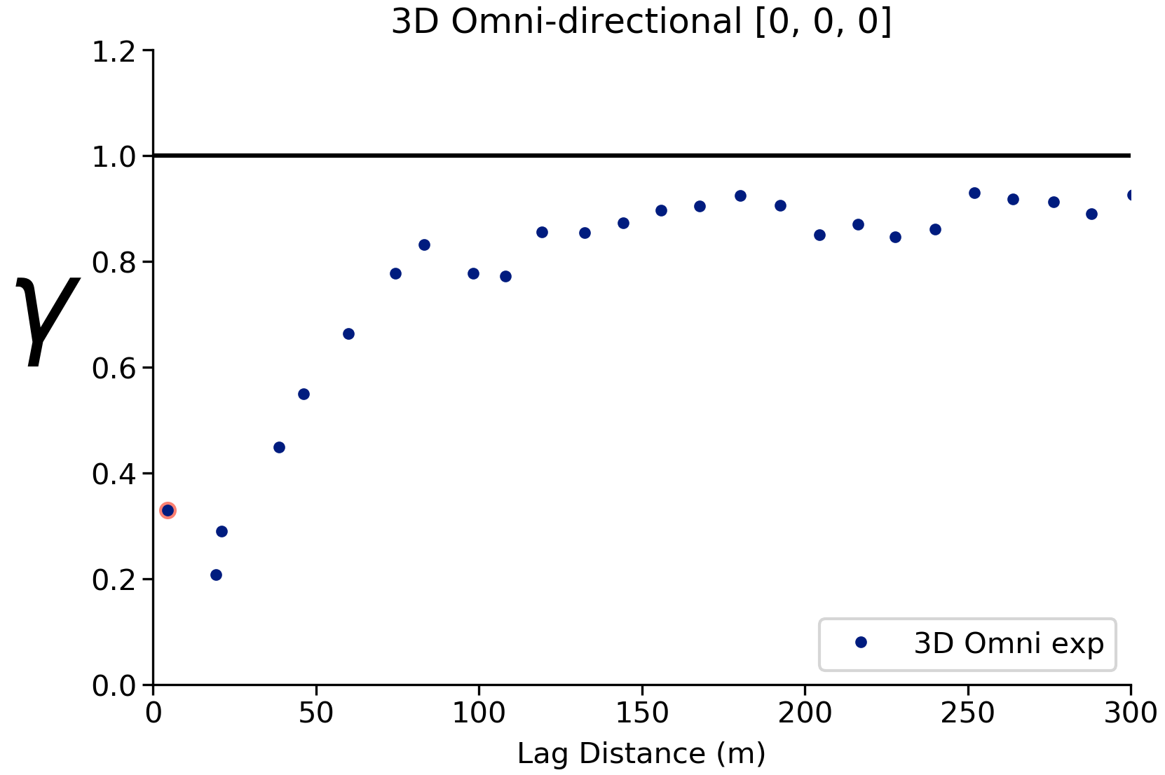
This variable is reasonably continuous, even with that first shitty point 😂:

Nearest Neighbor

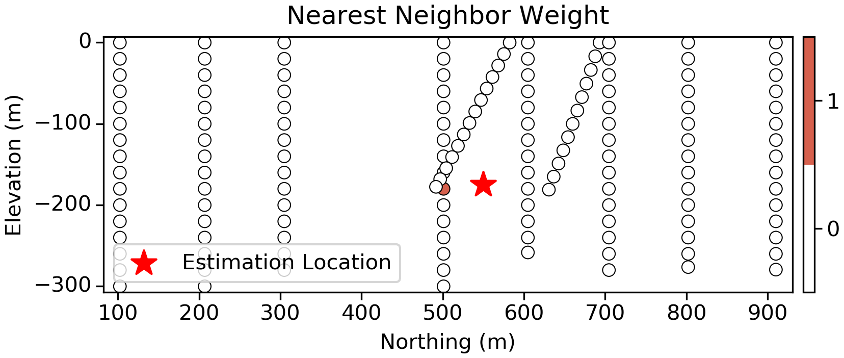
First up are Nearest-Neighbor (NN) weights. In this case we find the nearest sample and assign this single value to the estimation location:

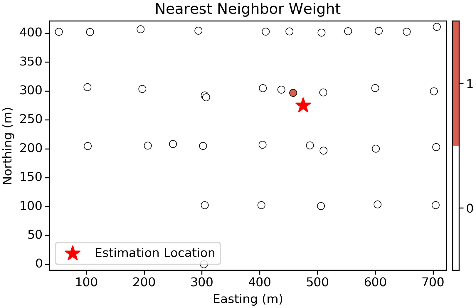
Considering the sampling pattern and the continuity observed in the variogram above, this approach is clearly limiting since there are other samples in the area that should probably have an influence on the estimated value. This limitation is especially worrying in the vertical slice (below) since there are many tightly spaced samples that we should consider to make an estimate, but only the single closest sample is considered:

Inverse Distance Squared

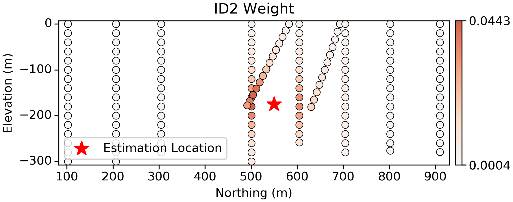
ID2 is a more reasonable approach that weights samples based on their distance to the estimation location. The weights are predictably high for samples closest to the estimation location, and approach 0.0 as the distance increases. Note that the weights are never zero, since $ \frac{1}{distance} $ is asymptotic as $ distance \rightarrow \infty$.

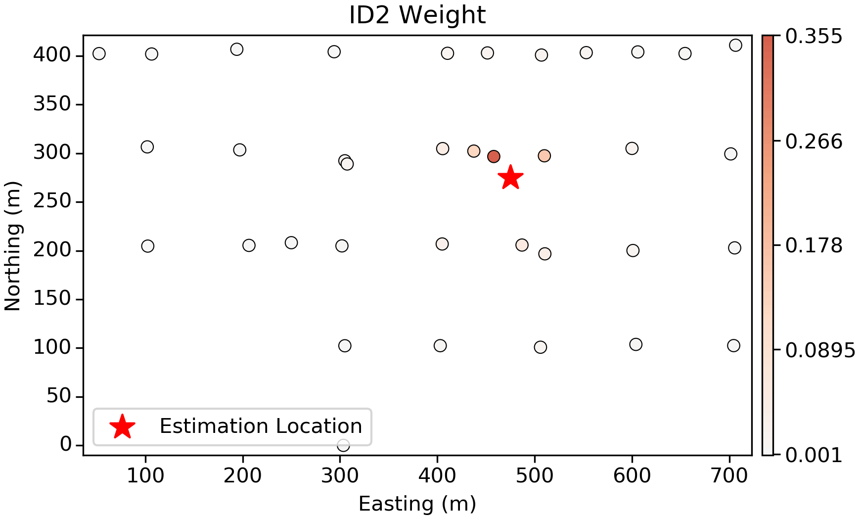
Both the plan view slice above and the vertical slice show predictable weights based on the position of the samples relative to the estimation location.

Simple and Ordinary Kriging

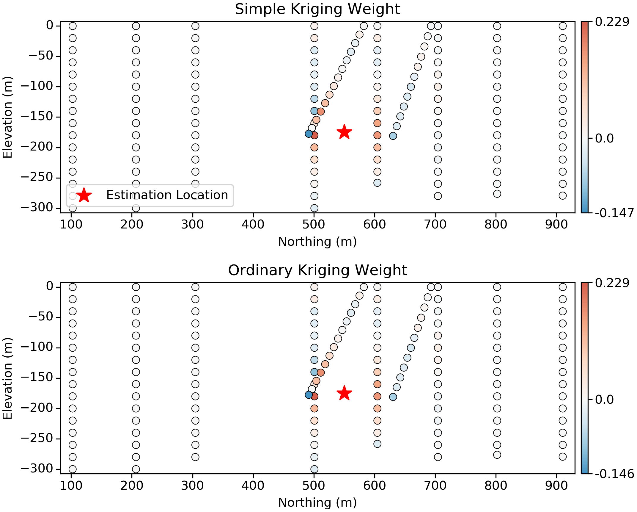
The kriging weights are calculated by specifying an optimality criteria. That is, we calculate weights to minimize the mean squared error (MSE) between the estimate and the unknown true value. As we mentioned previously, these weights are special since they consider both the position of the samples to the estimation location and the position of the samples to each other.

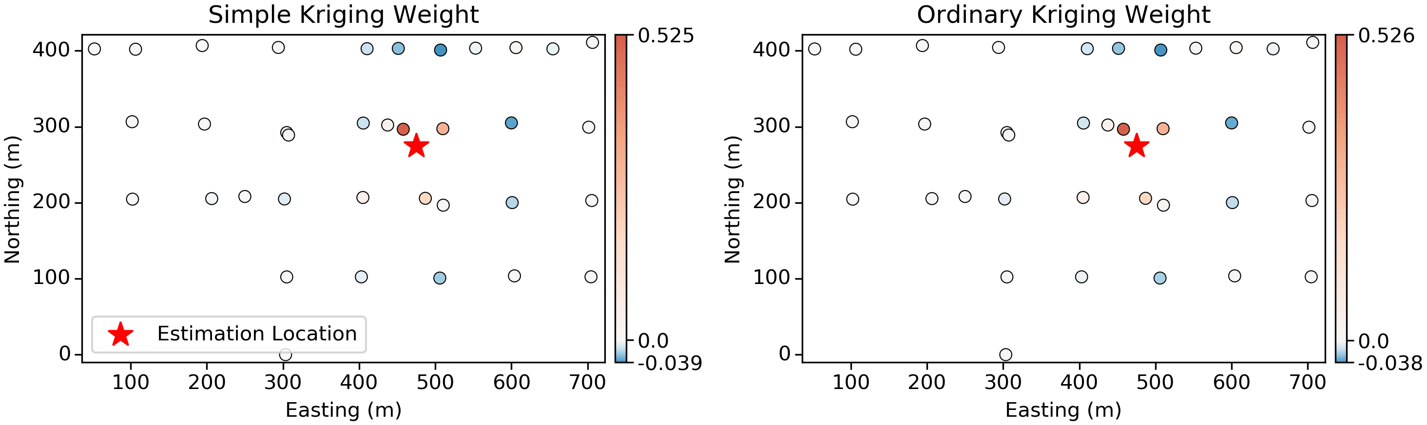
The kriging weights typically show “screening”; when two samples are close to one another, but one is closer to the estimation location than the other, the more distant sample will be “screened” with a low (and sometimes negative) weight. For example, in the above plots, the closest samples to the estimation location are given high-positive weight, with a select few samples in a sort of “outer ring” given a small negative weight.

Negative Kriging Weights??

Yeah, at first glance, negative weights seem strange… but they are a perfectly reasonable outcome of the kriging system of equations. It can help to think about it with a simpler data configuration:

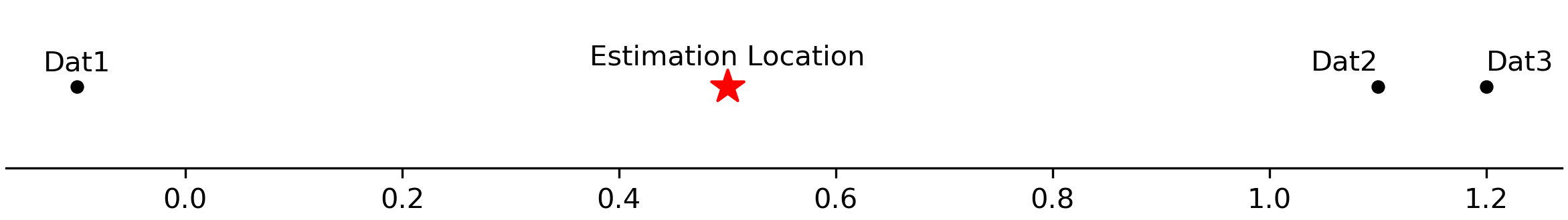
So in this case we have 3 sample locations and a single estimation location arranged in a 1-dimensional domain, spread across the x-axis. The spatial correlation matrix for this setup is shown below:

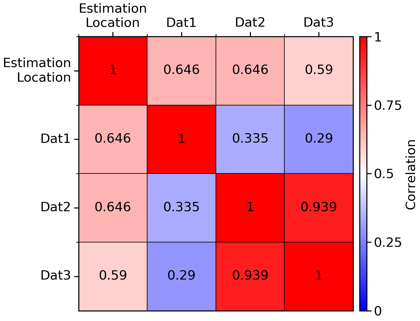
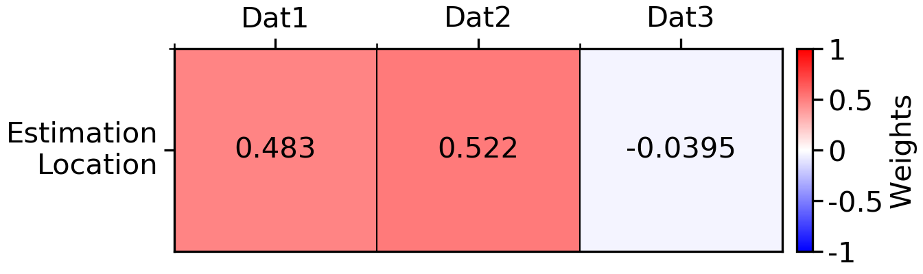
Locations 1 and 2 are equally correlated to the unsampled location at ~0.65 and have a (relatively) low correlation with one another (~0.34). Location 3 is slightly less correlated to the estimation location, but highly correlated to location 2. The simple kriging weights calculated for this configuration are:

And the ordinary kriging weights:

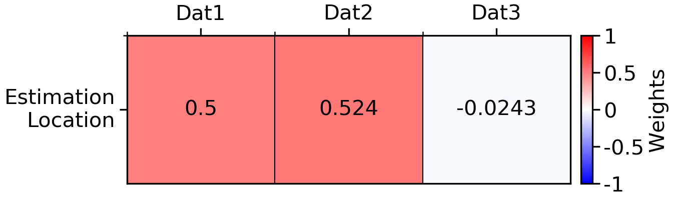
Interestingly, the weight of Dat2 is higher than Dat1 in both cases, and their difference is equal to the weight of Dat3. In effect, this is making sure the estimate calculated for the Estimation Location is an unbiased representation of the data surrounding it. It may help to think of this property as a type of declustering. If Dat3 did not exist, then the weights of Dat1 and Dat2 would be 50/50, as both data are the same distance from the Estimation Location along the same vector of continuity. But because Dat3 is present, is it fair to assign the geology that Dat2/Dat3 represents more weight than the geology that Dat1 represents, within the same estimation domain? In most cases, probably not. Weights calculated by ID2 would not consider this type of spatial redundancy. However, there is a point of diminishing returns, as with enough data density, the estimates calculated with Kriging, ID, and RBFs will effectively converge.

Back to the 2D example, the vertical slices below show how the data configuration can play into screening and negative weights. Significant screening is occurring here, with negative weights almost equal in magnitude to the positive weights that screen them. In practice, there are some special circumstances where negative weights can be problematic:

1. In nuggety deposits (such as Au, Ag) and,
2. With special data configurations (like below).

Now, imagine this was a nuggety gold deposit, where the gold value between even the closest samples can vary wildly, and a negative weight is given to a location that randomly has a high gold value relative to samples around it, we could end up with a negative estimate of the gold grade. Should we reset negative weights to zero? In my opinion, no. There are more sophisticated methods for treating these weights; the alternative is to let the negative weights happen and just reset negative estimates to zero. A better solution to this issue is to use multiGaussian kriging, where the Gaussian transformation is applied pre-estimation and in a post-processing step. Under those conditions it is impossible to estimate negative gold grades, and the negative weights are perfectly reasonable.

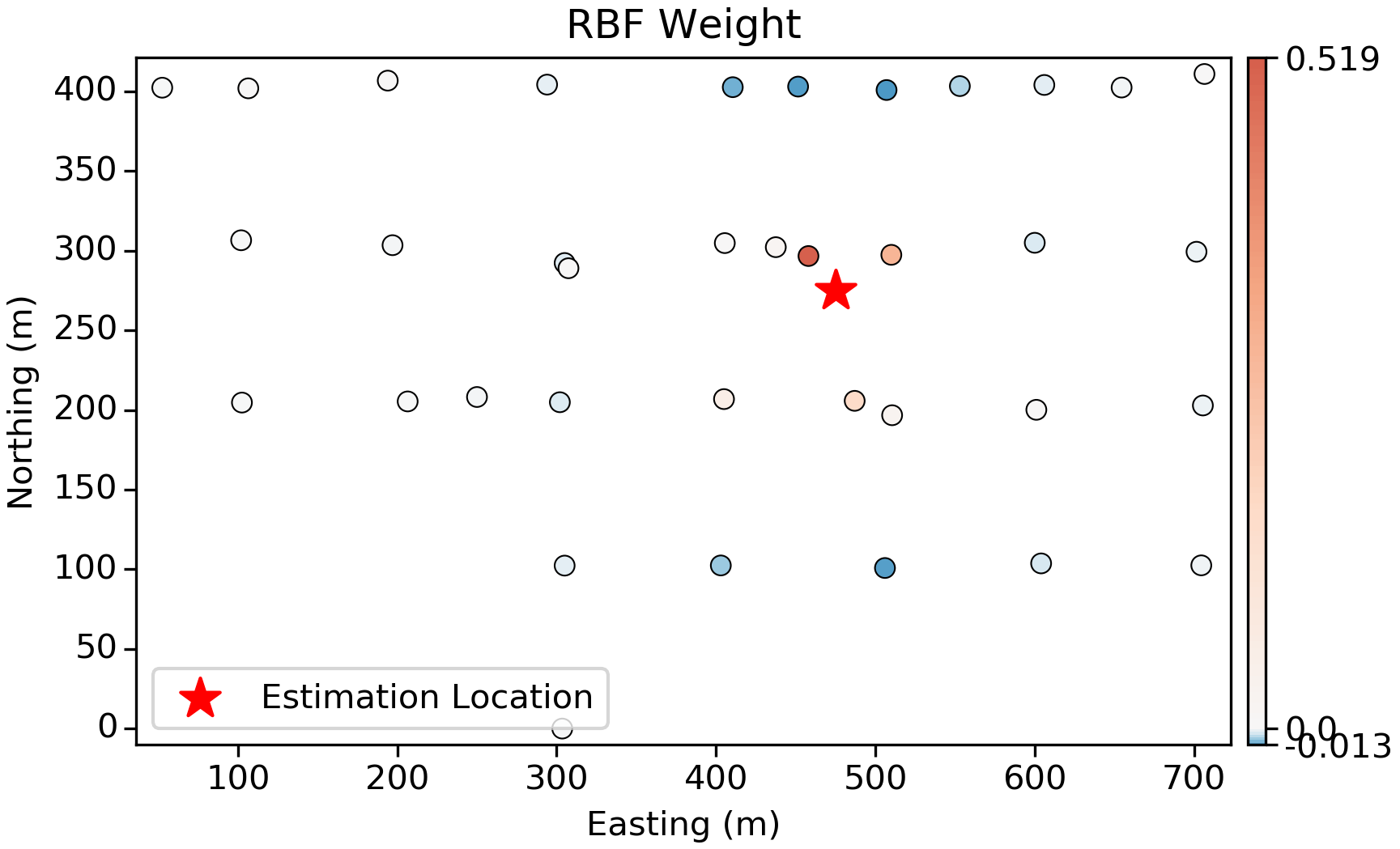
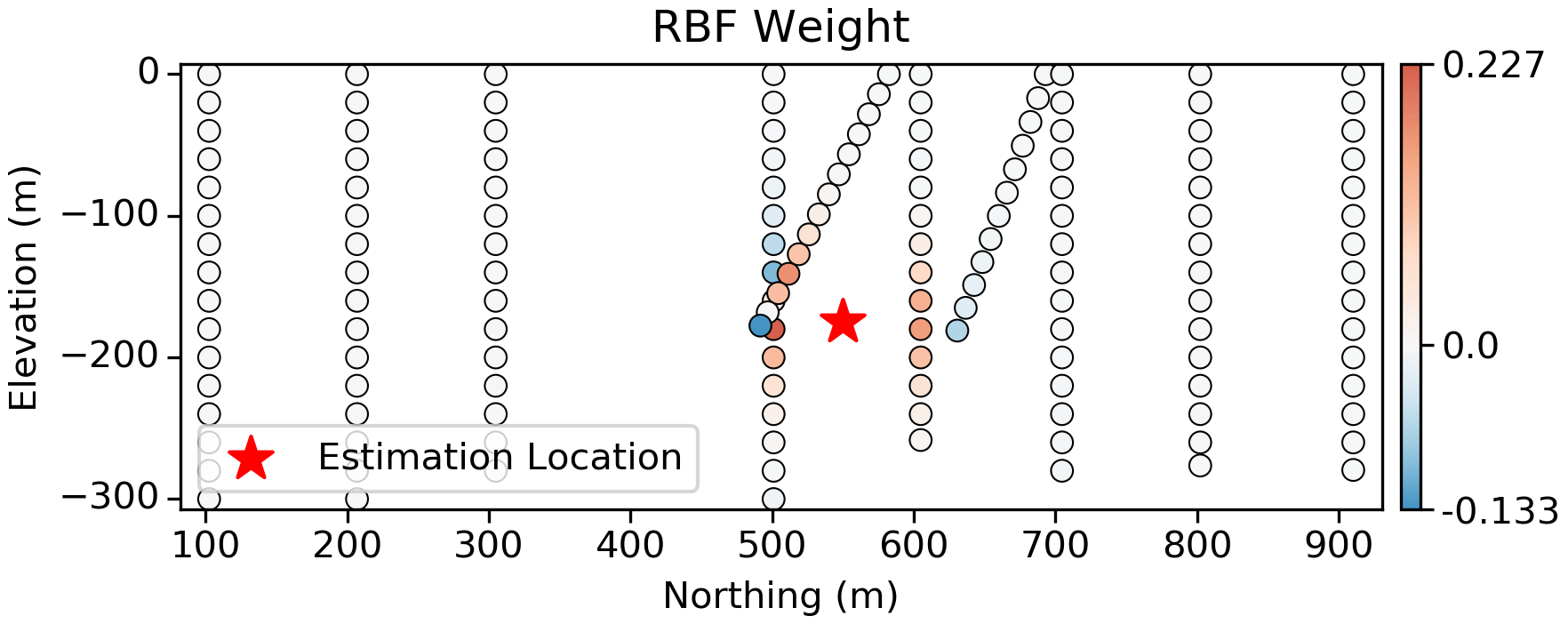
Radial Basis Functions

Weights calculated from radial basis functions (RBF) are similar to kriging. In this case a Linear kernel is used, which has no range parameters; we see the same screening with negative weights, but the magnitude of the negative weights is lower both in the plan view and vertical slices.

Summary

We have so many ways of weighting data to generate an estimate. None are wrong. Some are more applicable than others.

Regardless of what we choose, it’s always good to know how things are working, and to be aware of the little details that affect each method.