Rolling your own estimators in Python

Ryan Martin
Date : October 2, 2020

Categories : Kriging ,Estimators ,Python
Tags : Kriging ,IDW ,NN ,RBF

Difficulty : 🔥🔥🔥🔥 / 5

This post shows how to use Python to combine spatial searches, weight calculations and linear algebra to ‘scratch-bake’ our own IDW, Kriging, RBF and NN estimators. This post is implemented in a Jupyter notebook and is a prelude for the next post where we deep dive into specific differences in how each estimator is weighting the nearby data.

Disclaimer

I believe everyone in resource estimation should feel the joy of “rolling their own” estimator one day. It provides all kinds of understanding into the details that you just don’t get from commercial software, a textbook or a lecture. But, if you do decide to venture down this path, take great care if using your algorithms in “production settings”; you should well test your implementation or prefer well tested implementations… the code below is untested beyond these posts!

Introduction

The “batteries included” mentality of Python provides huge potential for exploring algorithms in geostatistics. What was once obfuscated behind decades old programming languages and compilers is now readily accessible to anyone who can work the Google machine. In this post we’ll focus on estimation and all the details of estimation. Recall from previous posts that estimating value in a spatial context comes down to choosing how to weight values from nearby locations. To implement an estimation algorithm we need to:

1. Calculate distance
2. Perform nearest-neighbor spatial queries
3. Calculate weights with specific formulas that might include linear systems of equations
4. Have some way to represent covariance functions (Kriging)
5. Have some way to represent basis functions (RBF’s)

Items 1-3 are common operations found in a few key Python libraries. Items 4 and 5 require a small amount of custom Python to get going. Let’s take a look at how we’d do it.

Distance Calculations

Distance calculations are found everywhere in science and computing. Unsurprisingly there are many easy to use and highly optimized libraries for calculating distances in Python. In our case we will consider the scipy.spatial.distance package and specifically the pdist and cdist functions.

Let’s say we have a set of locations stored as a matrix with N rows and 3 columns; each row is a sample and each column is one of the coordinates. The cdist and pdist functions cover two common cases of distance calculation. If we need a set of pairwise-distances - the distance from each sample to every other sample accumulated in a square matrix - then pdist is the function we’re looking for. Alternatively, if we have 1 location and we want distances from that location to some other set, we use cdist. Both options are demonstrated below:

from scipy.spatial.distance import cdist, pdist, squareform
compressed_dist_mat = pdist(data_locs)
square_dist_mat = squareform(pdist(data_locs))
dist_vector = cdist(estimation_loc, data_locs)

Anisotropy

Distances calculated above are isotropic - this is somewhat limiting for geostatistics since we usually have preferential continuity along certain orientations that we’d like to account for (e.g., geological distances being shorter than Cartesian distances). The trick is to use a rotation matrix, and pre-rotate and scale the whole problem into the new space that accounts for this geological distance. The only caveat is to make sure to rotate all possible locations to this new space before calculating any distances.

Nearest-Neighbor Queries

KDTree’s are a much better solution for querying locations in a local window. An excellent generalized implementation of this is found in sklearn.neighbors:

from sklearn.neighbors import KDTree
tree = KDTree(data_locs)
distances, indexes = tree.query(search_locations, k=k_nearest)

The result of a KDTree search is a set of k distances and indexes to the locations from the tree that are nearest to the location being searched. This is akin to performing cdist at each search location, sorting from smallest to largest, and keeping the records with the k-smallest distances. These are also isotropic, but the same pre-rotation trick is permissible here, too.

Mathematical Computations

If you’ve been around the Python world or have ever seen any kind of intro to Python, you’ve probably heard of Numpy. Numpy provides all kinds of base mathematical abstractions, like an “array” or “vector” (1D sequence of numbers) or “ndarray” or “matrix” (2+D ‘table’ of numbers). I’m not sure I’d get much out of Python these days without Numpy in my toolbelt.

The only special piece of Numpy that we’ll use is the linear algebra stuff from numpy.linalg.

Implementing Estimators

Spatial estimators of different types have several common steps. We have to do some preprocessing, search for locations, calculate weights and then calculate our estimate. A simple estimator prototype function might look like:

def estimate(
    data_locs, data_values, estimation_locs, k_nearest=45, **estimator_params
):
    data_values, data_locs = get_valid_inputs(data_locs, data_values)
    tree = KDTree(data_locs)
    dist, idxs = tree.query(grid_locs, k=k_nearest)
    weights = get_weights(dist, **estimator_params)
    estimate = np.sum(weights * data_values[idxs], axis=1)
    return estimate

Let’s break this down a little. The basic inputs are matrices of locations (N rows and 3 columns), some values to estimate from, and then some estimation parameters (k-nearest points, and estimator specific parameters) This function then does the following steps

Prepare the data (find valid inputs, create a KDTree for distances etc.)
Get the weights for the k_nearest points
Estimate your value!

And you thought this was going to be hard! ;-) Implementing different estimators comes down to implementing different types of weighting functions.

Nearest Neighbor

Nearest neighbor (NN) gives all the weight to the closest sample, and 0 weight to everything else. Since the KDTree search returns the k nearest locations, we simply ask the KDTree for 1 nearby location, then assign the value of that location to our estimate. The weighting function looks like:

def get_nn_weights(distance):
    weights = np.ones_like(distance)
    return weights

Inverse Distance Weighting

Recall that inverse-distance weighting (IDW) calculates weights that are inversely proportional to distance raised to some power. One possible way to implement this is shown below:

def get_idw_weights(distance, reg_const, power):
    weights = 1 / (reg_const + distance ** power)
    weights = weights / weights.sum(axis=1).reshape(-1, 1)
    return weights

In this case reg_const is a constant that ensures we don’t divide by zero, and power is the all important parameter for controlling the continuity; higher powers means more localized influence (akin to shorter range variograms and bullseyes). Some of the extra notation has to do with vectorized operations with Numpy… not important at this stage.

Kriging

Kriging adds some complexity since weights are calculated to minimize the mean squared error. The simple kriging weights are calculated from the normal equations:

$$ C_{ij} \lambda_i = C_{i\Box} $$

Where $C_{ij}$ is a square pairwise covariance matrix between $N$ locations found in a local window, $\lambda_i$ are the weights we are trying to solve for, and $C_{i\Box}$ is the covariance between the $N$ locations and the place we are estimating. An implementation for simple kriging (SK) weights might look like the following:

def get_simple_krige_weights(cov_func, data_locs, grid_data_dists):
    # Calculate the pairwise-distances
    square_data_data_dists = squareform(pdist(data_locs))
    # Convert distances to covariance
    Cij = cov_func(square_data_data_dists)
    Ciu = cov_func(grid_data_dists)
    # Solve for weights and return!
    weights = np.linalg.solve(Cij, Ciu)
    return weights

The final piece is that cov_func that converts distances to covariances. Recall the variogram model that captures spatial variability also defines a covariance function, which converts arbitrary distances to covariances. One possible way to implement covariance functions is to make different callable objects,

🔥 Warning: object oriented Python ahead !🔥

class Covariance:
    def __init__(self, max_range, nugget, sill=1.0):
        self.max_range = max_range
        self.nugget = nugget
        self.sill = sill

    def apply_diag(self, cov_mat):
        """Set the diagonal to the sill of the model"""
        if cov_mat.ndim == 2 and cov_mat.shape[0] == cov_mat.shape[1]:
            # set the diagonal to the sill
            cov_mat[np.eye(cov_mat.shape[0], dtype=bool)] = self.sill
        return cov_mat

class SphericalCovariance(Covariance):
    def __call__(self, distance):
        """Calculate Spherical Covariance from `distance`"""
        distance = np.asarray(distance) / self.max_range
        covariance = np.zeros_like(distance)
        idxs = distance < 1.0
        covariance[idxs] = (self.sill - self.nugget) * \
            (1.0 - distance[idxs] * (1.5 - 0.5 * distance[idxs] ** 2))
        covariance = self.apply_diag(covariance)
        return covariance

class ExponentialCovariance(Covariance):
    def __call__(self, distance):
        """Calculate Exponential Covariance from `distance`"""
        distance = np.asarray(distance) / self.max_range
        covariance = (self.sill - self.nugget) * np.exp(-distance)
        covariance = self.apply_diag(covariance)
        return covariance

So, let’s say we want to krige with a spherical covariance function with 150 range and no nugget:

cova_func = SphericalCovariance(150, 0.0)

To calculate the covariance at a certain distance, we ‘call’ our object like its a function:

c = cova_func(distance)

And then this can be passed directly into the weighting function, and easily swapped out for other covariance models:

weights = get_simple_krige_weights(cova_func, data_locs, grid_data_dists)

The ordinary kriging (OK) weight function is slightly more complex because we have an extra constraint:

def get_ordinary_krige_weights(cov_func, data_locs, grid_data_dists):
    # Get the number of nearby locations, the `k` from the spatial search
    k_nearest = grid_data_dists.shape[0]
    # Setup the left-hand-side covariance matrix for OK
    Cij = np.ones((k_nearest + 1, k_nearest + 1))
    Cij[-1, -1] = 0.0
    # Calculate distances and convert to covariances
    square_data_data_dists = squareform(pdist(data_locs))
    Cij[:-1, :-1] = cov_func(square_data_data_dists)
    # Setup the right-hand-side covariance, calc distance and convert
    Ciu = np.ones(k_nearest + 1)
    Ciu[:-1] = cov_func(grid_data_dists)
    # Solve for weights, and return!
    weights = np.linalg.solve(Cij, Ciu)[:-1]
    return weights

RBF

Radial basis function interpolators are global, which means all samples are used to make the estimate at all locations. This sounds kind of “brute force”, like calculating the distance to all locations from above, but the problem is formulated in such a way that weights are calculated once and then can be used to efficiently estimate at all estimation locations in the domain. Weights are found in a similar way to kriging:

$$ K_{ij} \lambda_i = z_i $$

In this case $K_{ij}$ is a square pairwise matrix of kernel values (similar-ish to covariance) for all $N$ locations, $\lambda_i$ are the weights, and $z_i$ are the data values at the sample locations. The main difference with kriging is the use of kernels/basis functions versus covariance functions. The kernels used in RBF interpolation are less restrictive than covariance functions, but in this framework, do a similar job to covariance. Implementing them as callable objects:

class LinearKernel:
    def __call__(self, distance):
        return distance

Interestingly, there are no parameters for a linear kernel; we give it a distance and it gives us the distance back. Putting this in terms of covariance, usually you give distances and get covariances that decrease with increasing distance (things are less related when further away). But this linear kernel has a higher value the further the sample is from the current location… this is a little counterintuitive… but it works just fine in practice!

The basic form of this estimator is slightly different because all the weights are calculated up front:

def rbf(data_locs, data_values, estimation_locs, kernel):
    # Prep the data
    data_values, data_locs = get_valid_inputs(data_locs, data_values)
    # Compute the pairwise kernel matrix
    Kij = kernel(squareform(pdist(data_locs)))
    # Solve for the weights
    weights = np.linalg.solve(Kij, data_values)
    # Allocate array for estimates
    ests = np.full(estimation_locs.shape[0], np.nan)
    for i, eloc in enumerate(estimation_locs):
        # Get the kernel-values est location to all data locations
        k = kernel(cdist(np.atleast_2d(eloc), data_locs))[0]
        ests[i] = np.dot(weights, k)
    ests[ests < 0.0] = 0.0
    return ests

Testing our Estimators

Of course, we need something to interpolate. Below is a simple domain with a single variable sampled along mainly vertical drill holes:

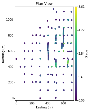
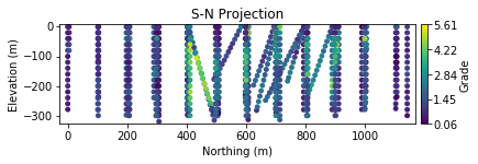
There is clearly some preferential sampling occurring in the central part of the domain that motivates declustering. The variable shows gradual spatial trends. Elevated values are intersected in the central to east portion of the domain:

The base case declustered histogram is shown below:

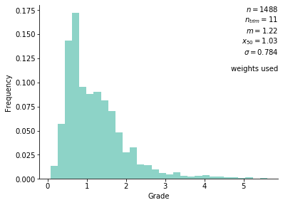
The distribution is weakly positively skewed with a small upper tail. Values from this dataset will be interpolated on a grid with ~255K nodes that span the drill hole locations.

Global Results

Let’s first take a peek at some global results by inspecting a histogram of estimated values. It’s important to have a representative reference distribution (read: take care of clustered sampling!):

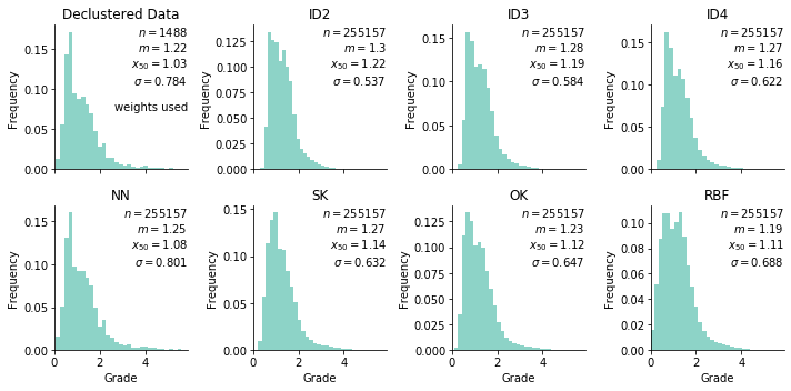
The big thing we’re checking here is the declustered histogram (top left) against the estimated models (rest). First off, the declustered mean is slightly over-estimated by everything but OK and is underestimated by RBF… Emphasis on slightly since all values are within 0.1 of the target declustered mean. All models except for NN have a lower standard-deviation resulting from well-known smoothing of these estimators.

Spatial Properties

In terms of the spatial properties, since we’re generating a single estimated model it comes down to visual inspection. South to North slices are shown below:

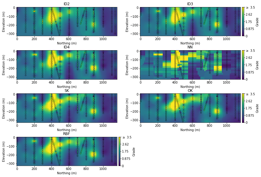
The inverse-distance models achieve the overall goal - a smooth interpolation of the underlying variable. The NN model generally captures the overall areas of elevated grade, but the artifacts are jarring. The SK, OK and RBF models are very similar - smooth and consistent…

Differences between the methodologies are further visible on a plan-view slice, notably the ID4 method is kind of starting to resemble the NN model:

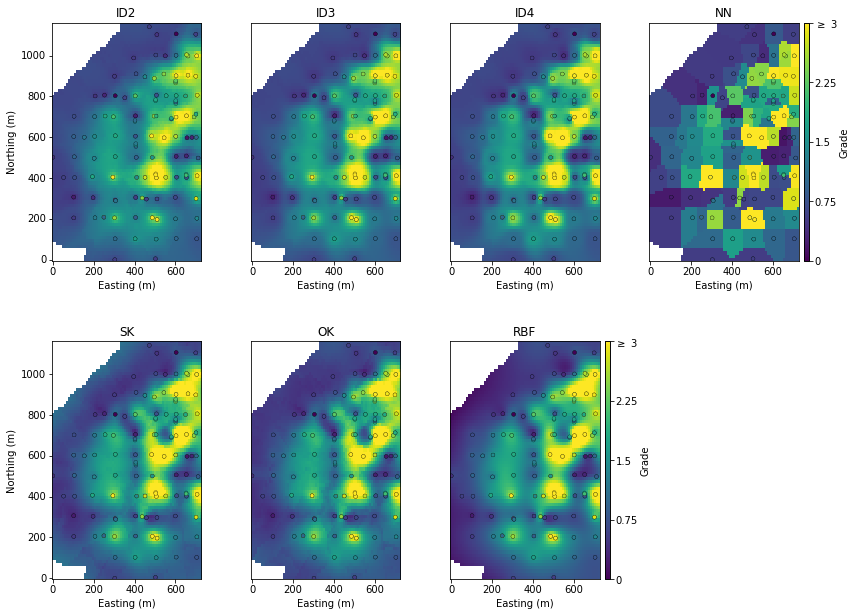
The only other thing that stands out are differences between the SK and OK models at the periphery beyond the influence of data (far left in the plan view SK model above). Beyond the influence of data the SK model would tend towards the global declustered mean, which will elevate local estimates relative to the actual value of the nearest data. OK on the other hand will re-estimate the local mean, which is exactly what is observed out to the edge of the model.

Summary

So, this post was pretty code heavy… I’ve shown how to use existing Python libraries to implement our favorite geostatistical algorithms… but, this post is mostly meant as a precursor to the next entry in this saga where we look at the weights given to nearby data by each algorithm and try to make sense of the differences and implications.