Data Spacing is the Social Distancing your Data Needs
TL;DR
Among all the hard lessons we learned during this pandemic perhaps the most important one is that social distancing saves lives. In mining, data spacing saves money, a lot of it. You may be interested in improving your resource classification, mine planning, or reducing global and local uncertainty; and most importantly, you want that to fit in your budget. That is when data spacing studies shine. Coupled with uncertainty models, data spacing studies provide a manner to optimize the information you get out of drilling. Understanding data spacing is an important step to make better decisions before is too late to change things.
Introduction
Here is a cliché, data spacing is a measure of data availability, and it measures the average spacing of nearby data. That is a bit obvious and boring to be honest. However, it becomes exciting and interesting when data spacing is calculated at high resolution models and combined with the assessed uncertainty for decision making. Let us start with data spacing and then I will cover some measures of uncertainty after.
Data Spacing
The LMC posts are not like your social media posts where you post online the same photo across different platforms for the same people to see. We are lazy, and laziness leads to efficiency. There is no need to duplicate content, you can find the details of data spacing calculation and concepts in this Geostatistics lesson I wrote a few years ago: http://www.geostatisticslessons.com/lessons/dataspacing. Let me summarize the key concepts for you, though:
- “Data spacing” is a measure of local data density, which can be calculated in several different ways for any drilling configuration, but it is often linked to regularly sampled and equally spaced drilling
- The calculation is easy for equally spaced drilling that are perpendicular to the plane of greatest continuity
- Drilling is often complex and irregular. In such cases you should calculate the data spacing locally at the same resolution of your resource model
- If your data is aligned in the same direction and perpendicular to the plane of greatest continuity, the calculation is simplified to a 2D case
- 2D calculation of data spacing requires either the number of data to search for or an area to find data in. You freeze one and calculate the other I suggest you freeze the number of data to search for and calculate the area to find them
- 3D cases involve the volume to search for data or the number of data to search for, in addition to the composite length. I suggest you freeze the volume – I often use an ellipsoid search – and calculate the number of data that falls within it
When calculating the data spacing keep in mind that you need to choose the calculation parameters considering the many transition zones of your data. That is, you must choose a reasonable set of parameters such that you identify transitions between sparsely and densely sampled areas of your deposit without excessive smoothing. For this reason avoid using the variogram range. The variogram is an overfitted tool that does not inform on transition zones and a difficult one to fit.
Combining the calculated data spacing with measures of uncertainty for mineral classification is a great combo. Let us get into measures of uncertainty.
Uncertainty
You cannot measure what you do not know! That is probably the easiest concept to understand when dealing with uncertainty, and yet, the most confusing in Geostatistics (and other fields). If you understand and can measure the uncertainty then it is no longer uncertain (wtf 🤨). Uncertainty is model dependent and all you can do is assess the uncertainty in your model. With that in mind, there are measures of uncertainty that you can calculate to assess the uncertainty in your model (confusing eh?). Let us not get lost in concepts and let us focus on the practicality of things.
You should assess the uncertainty with geostatistical simulation. And that is bad news for those out there who have been using kriging variance all these years. Here is why. Among many factors, including those that remain unknown for the modeler, and therefore are not captured by the model itself, the uncertainty at a location depends on the nearby data used for conditioning, the variogram function, the geological boundaries, the support of the data, the distribution of the data – and that involves how data is logged or flagged in the wireframes, declustering weights, capping, stationarity – the proportional effect and proximity to transition zones, the quality of data (drilling types), the resolution of the model, etc. … Now get all that and throw it in the garbage and replace it with kriging variance, that accounts only for the data configuration. That is stupid!
A common measure of uncertainty from simulation is the probability to be within a percentage of the simulated mean, which is briefly talked about here. To calculate it, start by taking the average of all values simulated at a location (often called an estimation type mean or E-type mean). You want to do this on a scale of relevance, e.g., the SMU. Then loop over all the simulated values and count the number of times that a simulated value falls within a percentage of the E-type mean. This measure of uncertainty is easy to calculate and interpret. For example, if I generate 100 realizations of gold grade with a simulated mean of 8 g/t and I tell you that the probability of gold grade to fall within 15% of the mean is 80%, it means that the simulated grade was within 6.8 g/t and 9.2 g/t in 80 realizations.
Combining Spacing and Uncertainty
The figure below was taken from my M.Sc. thesis, page 35, and it shows the typical shape of a data spacing versus uncertainty curve when plotting this measure of uncertainty. The uncertainty curve of your deposit might not look exactly like this one, in fact, they come in a wide range of shapes. You get the point though, you drill more you solve a scale of the variability. The rate that the uncertainty changes varies and controls the shape of the curve.
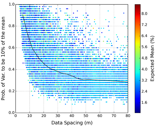
Each dot in the plot represents the calculated data spacing and the assessed uncertainty in a SMU. Use a regression algorithm to calculate the black line: the expected uncertainty curve. Then read the information from the curve by literally drawing lines that touch the curve in both axes. For example, you would need to drill at a 10m spacing to achieve a level of precision of 10% around the mean at 80% of the times. Note the obvious, you need to drill at a much smaller spacing to achieve a high level of confidence in your estimates.
Keep in mind that the uncertainty is scale dependent. When block averaging your simulation the high and low values are averaged out and the uncertainty “decreases”, that is, you can expect the uncertainty curve to go up! In other words, the data spacing required to achieve the same level of uncertainty increases with the scale of the measurements.
Consider now the framework above for resource classification. It is a powerful combo. You now have a measure of data availability that is easy to communicate! You now have a fairly straight forward measure of the uncertainty that is linked to both drill spacing and modelling scale and can support your point, for example, “drilling at X spacing we can expect the SMU grade to be within Y% of the mean Z% of the time”, where X, Y, and Z are variables read from the data spacing versus uncertainty plot.
Going further, you could use this information for mineral classification. Here is an example. You assess the uncertainty at different production scales. Classify the SMUs as measured or indicated based on the probability of their grades to be within 10% of the mean at least 80% of the times for quarterly and yearly production volumes, respectively. Use the calculated uncertainty curves for the respective scales to identify the data spacing required to achieve a desired level of uncertainty.
Do It Right
To summarize, do it right. Forget kriging variance, go for simulation. Calculate the data spacing avoiding artifacts, be fair with your search parameters and avoid using the variogram range. Use the measure of uncertainty that you are familiar with and comfortable making decisions with. Put them together in a data spacing and uncertainty curve and calculate the uncertainty curve. Remember, uncertainty is model and scale dependent. Connect the dots and you will have a good estimate of the data spacing needed to achieve a level of confidence. If possible, combine both for resource classification, it’s a good combo.
If you want to know more about data spacing, I recommend starting with the literature that I posted in the end. There is a lot more to read out there and I apologize to those whose names and work are not mentioned here. This post needs to be short and cannot fit everything that involves this exciting topic.
To Dig a Bit More
-
Cabral Pinto, Felipe A. & Deutsch, Clayton V. (2017). Calculation of High Resolution Data Spacing Models. In J. L. Deutsch (Ed.), Geostatistics Lessons. Retrieved from http://www.geostatisticslessons.com/lessons/dataspacing
-
Silva, Diogo Figueiredo Silva, Mineral Resource Classification and Drill Hole Optimization Using Novel Geostatistical Algorithms with a Comparison to Traditional Techniques. M.Sc. Thesis, University of Alberta, 2015. Retrieved from https://search.library.ualberta.ca/catalog/7087403
-
Wilde, Brandon Jesse, Data Spacing and Uncertainty. M.Sc. Thesis, University of Alberta, 2010. Retrieved from https://search.library.ualberta.ca/catalog/4853514
And finally if you really want to dive deep. You can look through my thesis. Just be forewarned because well…. It’s a thesis. Nuff said. Not for the faint or lazy at heart.
- Cabral Pinto, Felipe A., Advances In Data Spacing and Uncertainty. M.Sc. Thesis, University of Alberta, 2016. Retrieved from https://search.library.ualberta.ca/catalog/7646909